

Dynamics of seasonal and interannual variability of the ocean bottom pressure in the Southern Ocean
-
Abstract: Seasonal and interannual variability of ocean bottom pressure (OBP) in the Southern Ocean was investigated using Gravity Recovery and Climate Experiment (GRACE) data and a Pressure Coordinate Ocean Model (PCOM) based on mass conservation. By comparing OBP, steric sea level, and sea level, it is found that at high latitudes the OBP variability dominates the sea level variability at seasonal-to-decadal time scales. The diagnostic OBP based on barotropic vorticity equation has a good correlation with the observations, indicating that wind forcing plays an important role in the variability of the OBP in the Southern Ocean. The unique interannual patterns of OBP in the Southern Ocean are closely associated with El Niño-Southern Oscillation (ENSO) and Southern Annular Mode (SAM). Regression analysis indicates that ENSO and SAM influence the OBP through altering the Ekman transport driven by surface wind. The leading pattern of OBP from PCOM are very similar to observations. Sensitive experiments of PCOM show that surface wind forcing explains the observed OBP variability quite well, confirming the importance of wind forcing and related oceanic processes. In the eastern South Pacific, the averaged OBP shows a decrease (increase) trend before (after) 2011, reflecting the reverse trend in westerly wind. In the South Indo-Atlantic Ocean, the averaged OBP has a weak increase trend during 2003–2016.
-
Key words:
- ocean bottom pressure /
- Southern Ocean /
- interannual variability /
- PCOM
-
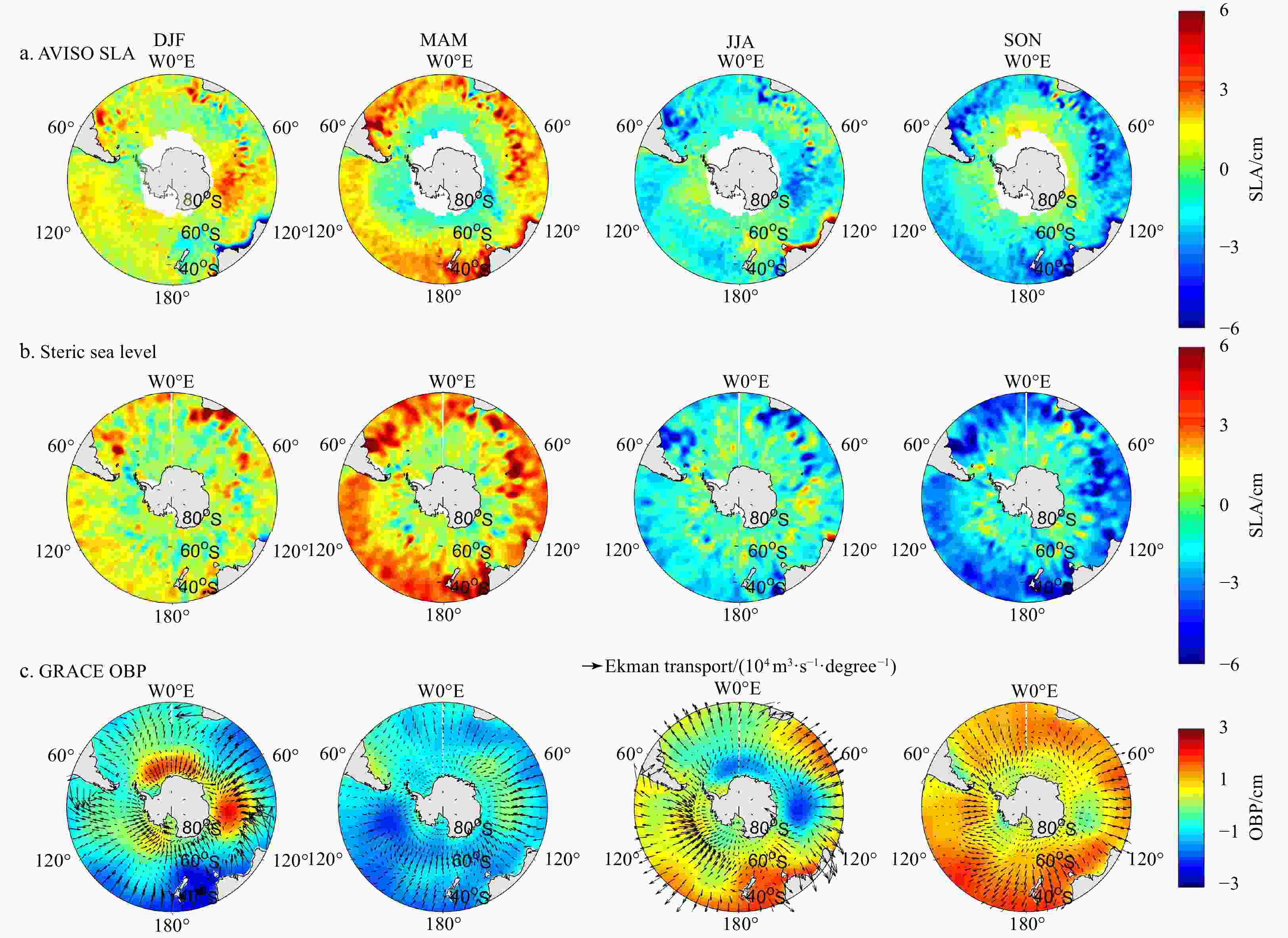
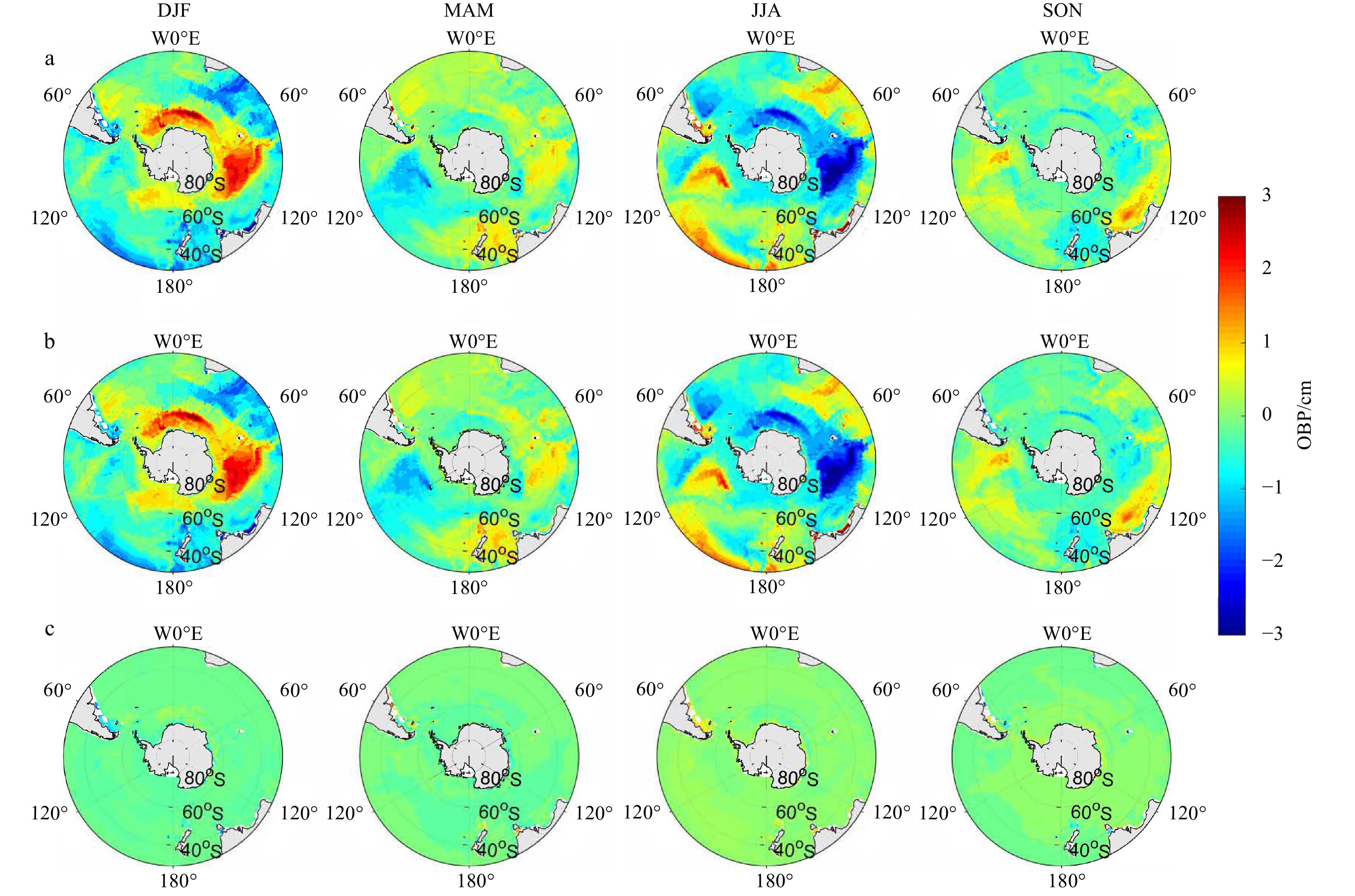
Figure 1. Seasonal variability of AVISO SLA (top, a), steric sea level (middle, b), and GARCE OBP (bottom, c) in the Southern Ocean for the period of 2004–2016 (color shading, in unit of cm). From left to right, each column represents austral summer (DJF, December, January and February), autumn (MAM, March, April and May), winter (JJA, June, July and August), and spring (SON, September, October and November), respectively. The vectors in c represent Ekman transport anomaly (in unit of 104 m3/(s·(o)) calculated from ERA-interim. Climatological annual mean has been removed.
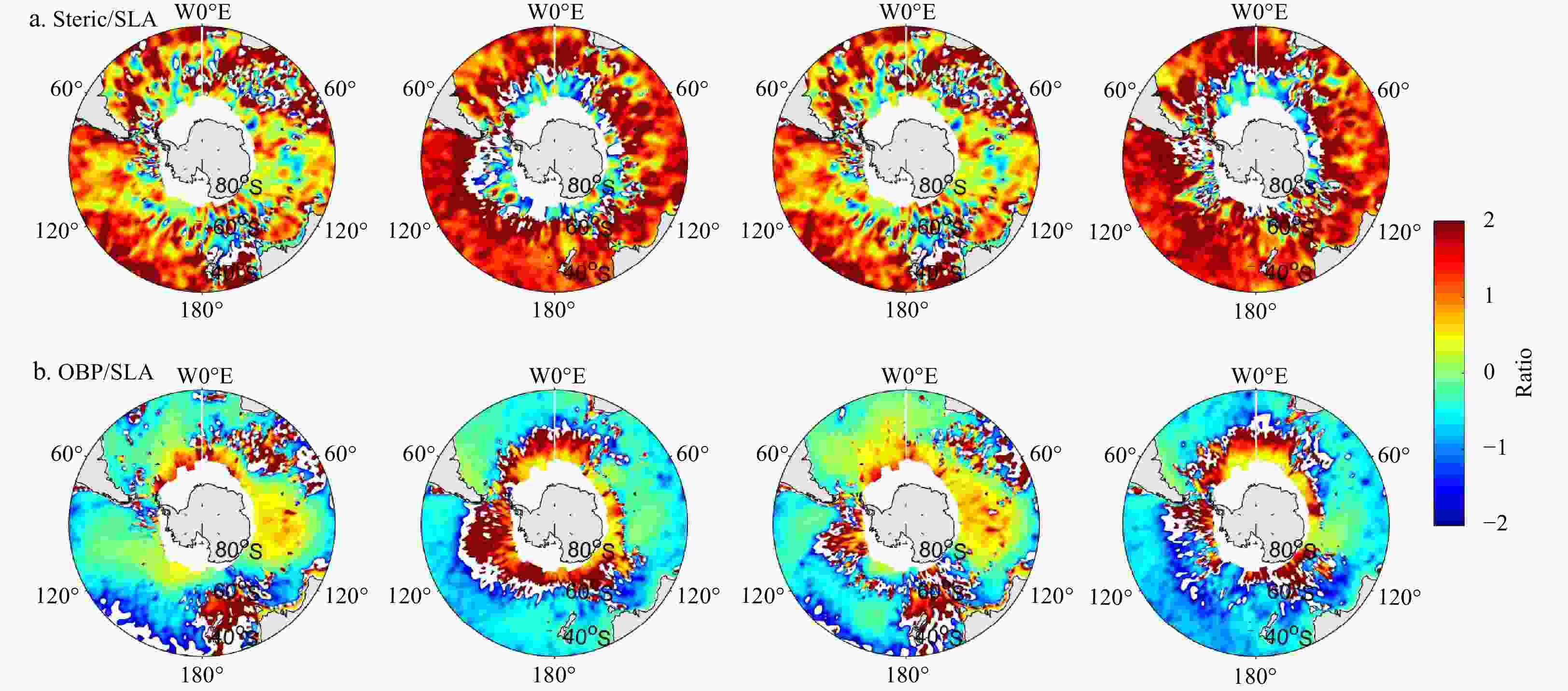
Figure 2. Ratio of steric sea level to sea level anomaly (a), and ratio of ocean bottom pressure to sea level anomaly (b).
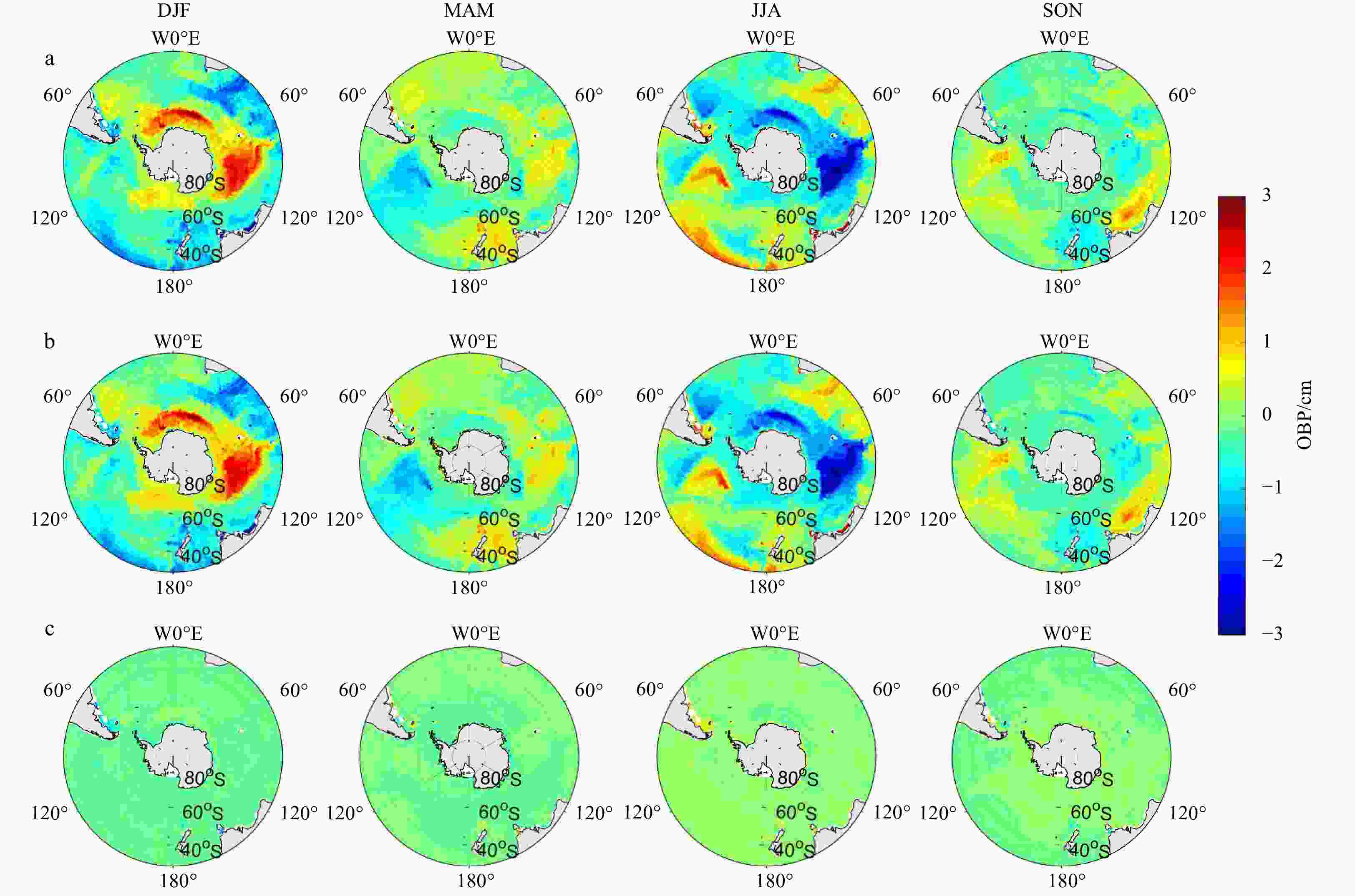
Figure 3. Seasonal variability of OBP (in unit of cm) obtained from PCOM runs: a. in control run (Exp. 1), b. without air pressure forcing (Exp. 2), c. without wind forcing (Exp. 3) averaged in austral summer (DJF, December, January and February; first column), autumn (MAM, March, April and May; second column), winter (JJA, June, July and August; third column), and spring (SON, September, October and November; fourth column) in the Southern Ocean from 2004 to 2016. Climatological annual mean has been removed.
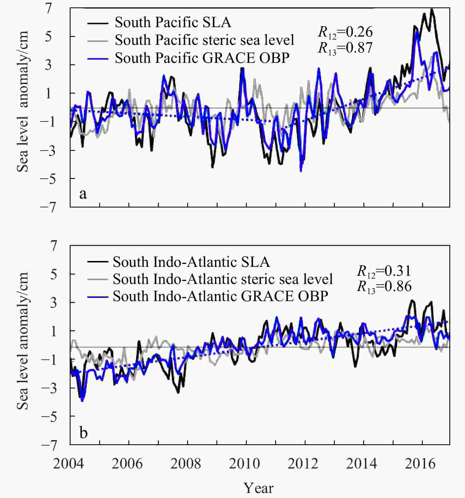
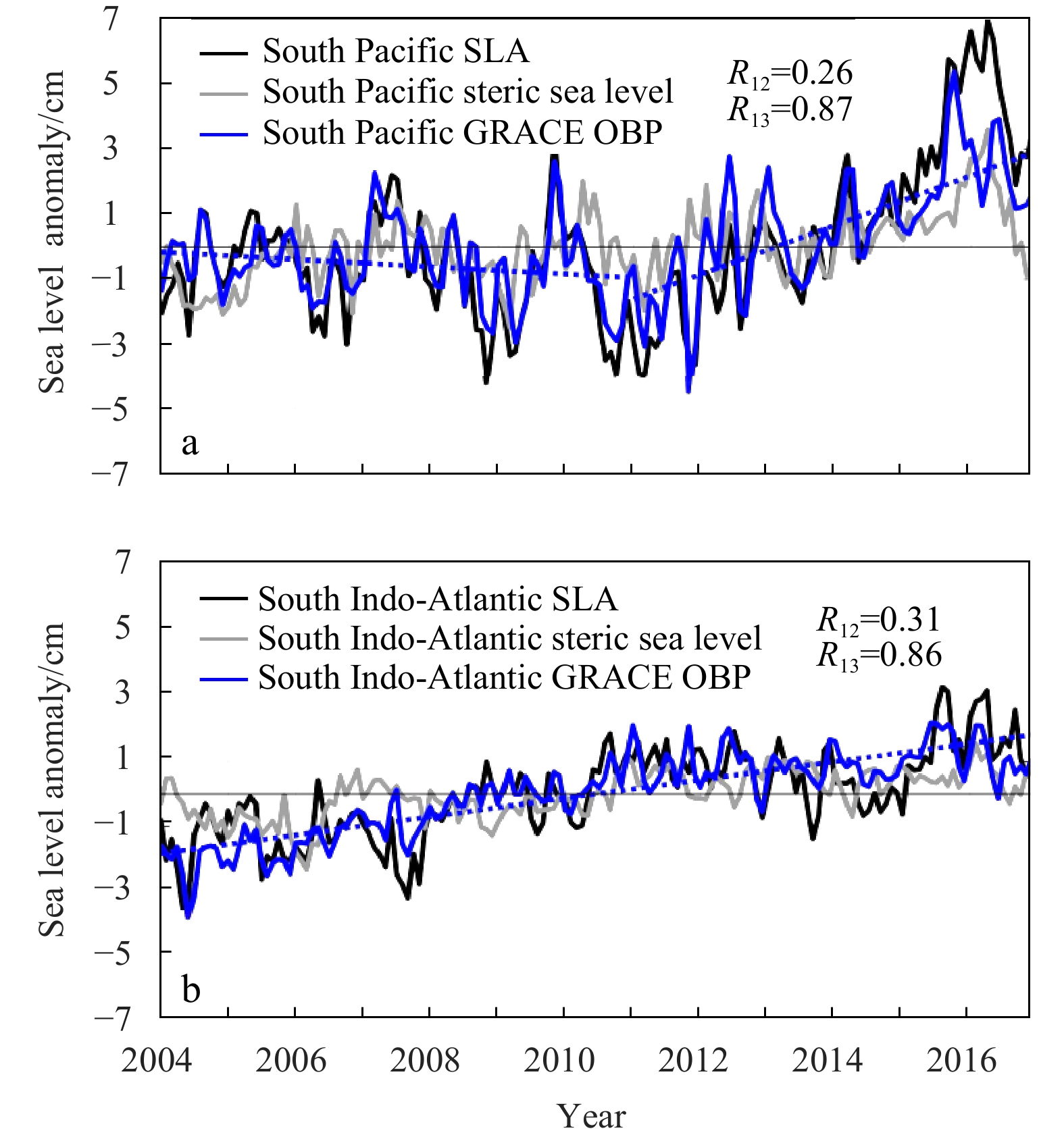
Figure 4. Time series of GRACE OBP anomaly (solid blue lines), SLA (solid black line), steric sea level anomaly (solid gray line) averaged in the South Pacific (40°–60°S, 150°–90°W) (a) and in the South Indo-Atlantic Ocean (40°–60°S, 60°W–120°E) (b) from 2004 to 2016. The anomalies are calculated by subtracting climatological annual cycle. The linear trends of GRACE OBP are displayed as blue dashed lines. In a, R12 is the correlation coefficient between South Pacific SLA and South Pacific steric sea level, and R13 is the correlation coefficient between South Pacific SLA and South Pacific steric GRACE OBP. In b, R12 is the correlation coefficient between South Indo-Atlantic SLA and South Indo-Atlantic steric sea level, and R13 is the correlation coefficient between South Indo-Atlantic SLA and South Indo-Atlantic steric GRACE OBP.

Figure 5. Time series of GRACE OBP anomaly (black lines), OBP anomaly reconstructed from wind forcing (pink lines) and topographic (topo) effect (blue lines) and sum of two terms (gray lines) averaged in the eastern South Pacific (40°–60°S, 150°–80°W) (a), the South Atlantic (40°–60°S, 60°–0°W) (b) , and the South Indian Ocean (40°–60°S, 30°–120°E) (c) from 2003 to 2016. The blue dashed lines are the trend of the GRACE OBP time series. The unit of the y-axis is cm. The anomalies are calculated by subtracting climatological annual cycle. In a, R14 is the correlation coefficient between South Pacific wind curl and South Pacific GRACE, R24 is the correlation coefficient between South Pacific topo and South Pacific GRACE, and R34 is the correlation coefficient between South Pacific wind curl+topo and South Pacific GRACE. In b, R14 is the correlation coefficient between South Atlantic wind curl and South Atlantic GRACE, R24 is the correlation coefficient between South Atlantic topo and South Atlantic GRACE, and R34 is the correlation coefficient between South Atlantic wind curl+topo and South Atlantic GRACE. In c, R14 is the correlation coefficient between South Indian wind curl and South Indian GRACE, R24 is the correlation coefficient between South Indian topo and South Indian GRACE, and R34 is the correlation coefficient between South Indian wind curl+topo and South Indian GRACE.
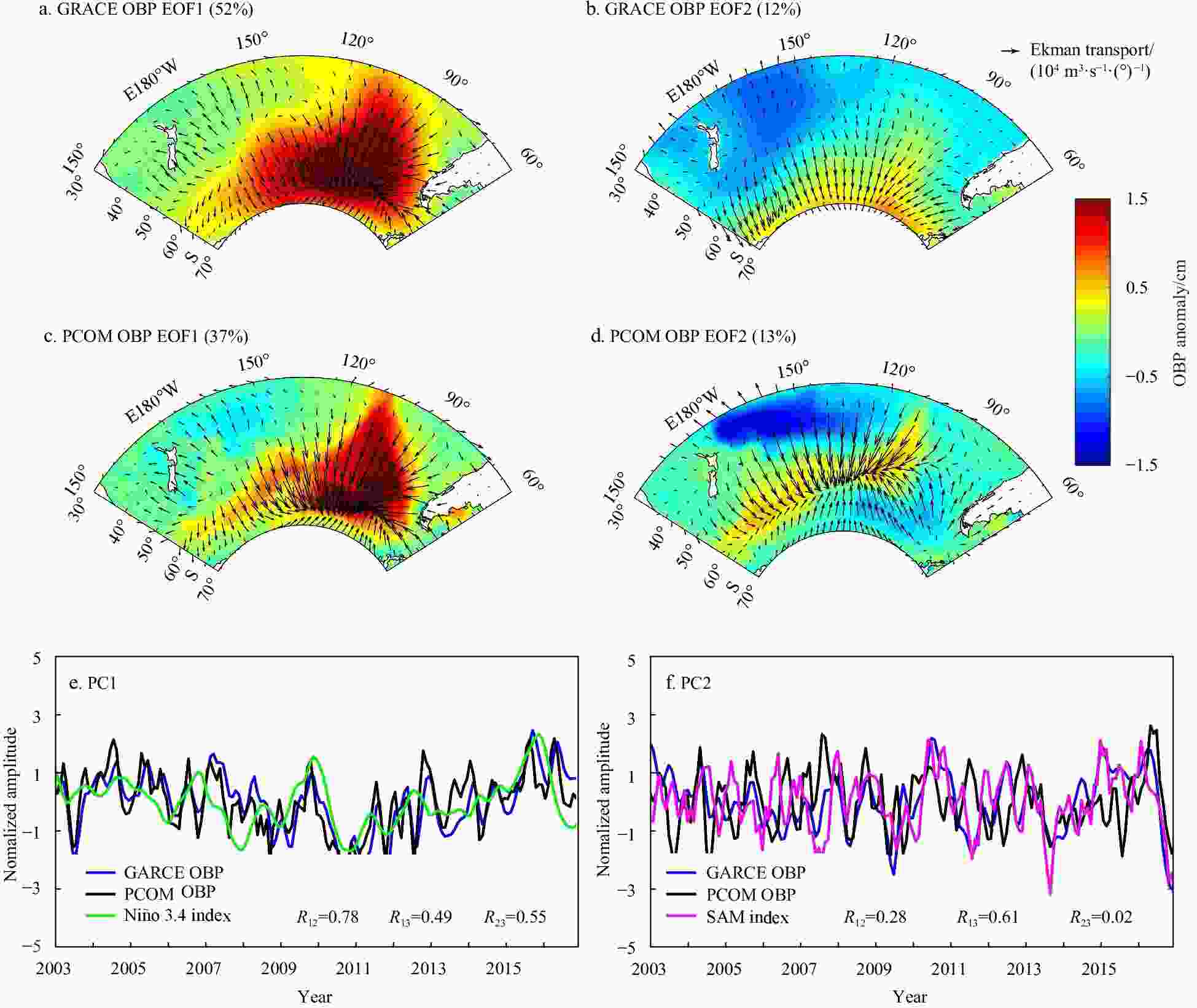
Figure 6. The spatial structures of the first EOF mode (a) and the second EOF mode (b) of the GRACE OBP (shade; cm) in the South Pacific Ocean from 2003 to 2016, and the spatial structures of the first EOF mode (c) and the second EOF mode (d) of the PCOM OBP (shade; cm) in the South Pacific Ocean from 2003 to 2016, and the rincipal component (PC) time series of the first EOF mode (e) and the second EOF mode (f). The green line in f represents the Niño 3.4 index. The pink line in f represents the SAM index. The vectors denote Ekman transport (104 m3/(°)) regressed on to each time series. Monthly climatology has been removed before EOF analysis.
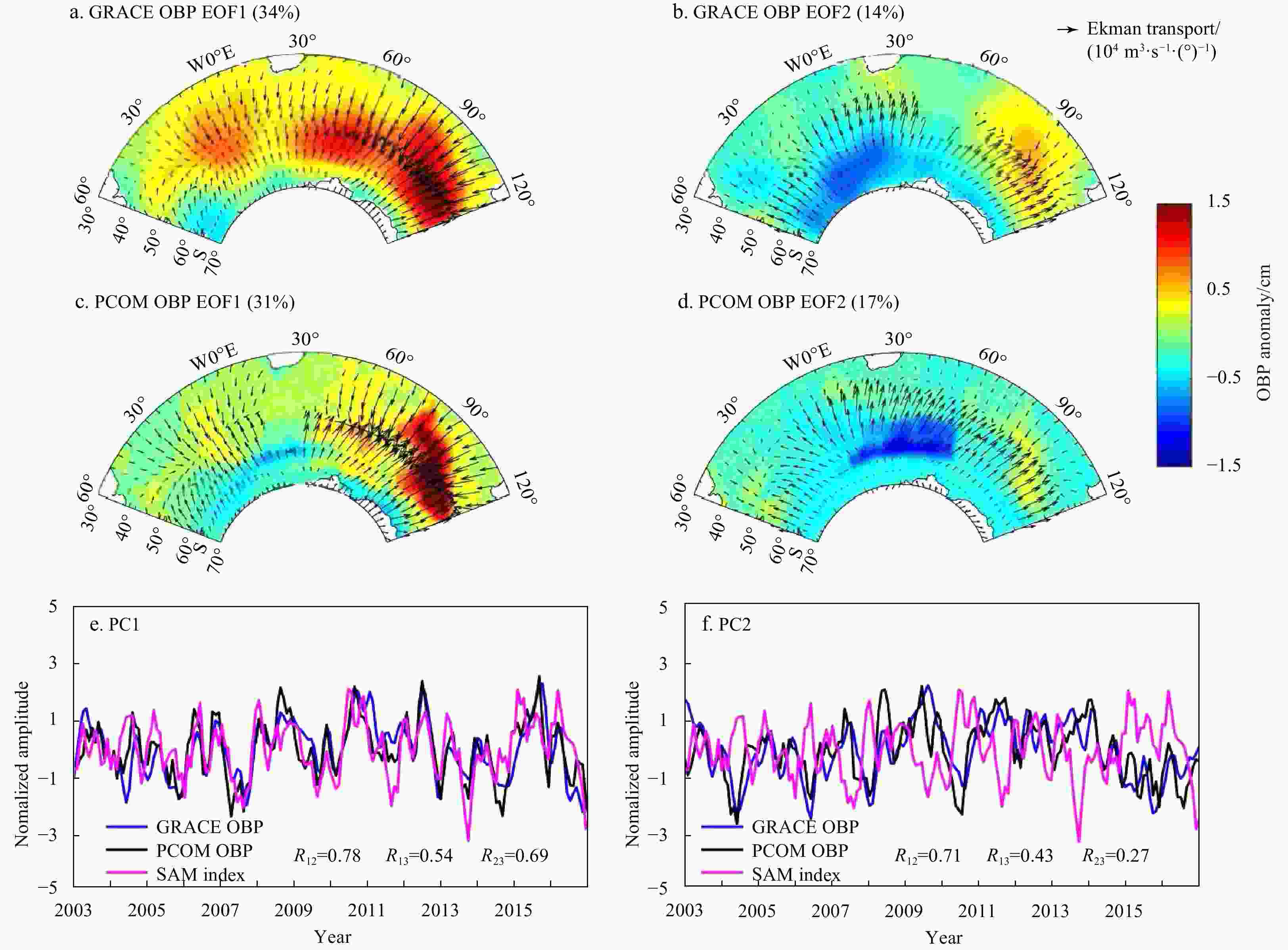
Figure 7. The structures of the first EOF mode (a) and the second EOF mode (b) of the GRACE OBP (shade; cm) and the spatial structures of the first EOF mode (c) and the second EOF mode (d) of the PCOM OBP (shade) in the South Indo-Atlantic Ocean from 2003 to 2016, and the principal component (PC) time series of the first EOF mode (e) and the second EOF mode (f). The pink lines in e and f represent the SAM index. The vectors denote Ekman transport (m3/(°)) regressed on to each time series. Monthly climatology has been removed before EOF analysis.
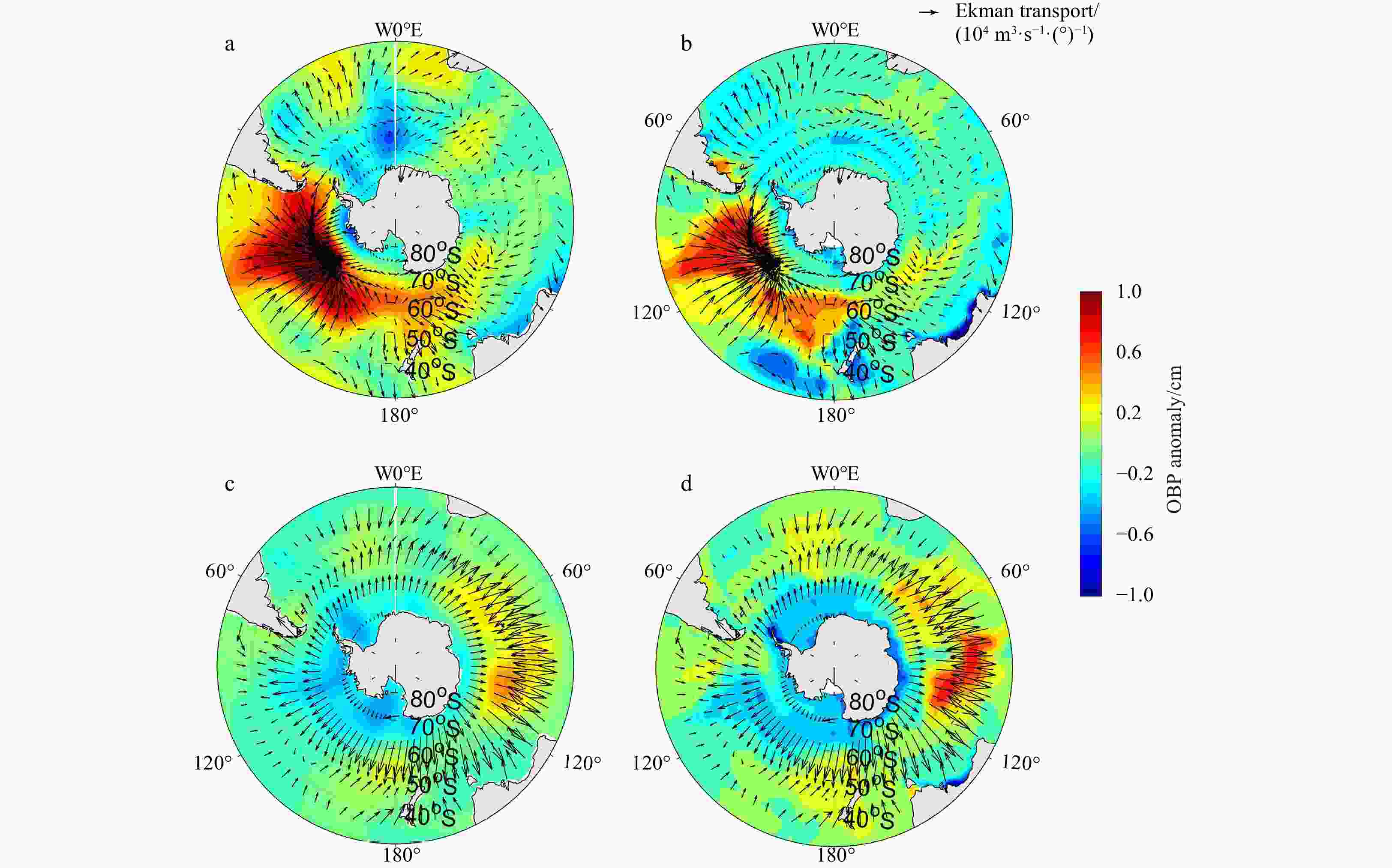
Figure 8. GRACE OBP anomaly (shading) and Ekman transport anomaly (vectors) regressed onto Niño 3.4 index (a) and SAM index (b) and PCOM OBP anomaly (shading) Ekman transport anomaly (vectors) regressed onto Niño 3.4 index (c) and SAM index (d) from 2003 to 2016. Ekman transport anomaly data are from ERA-Interim.
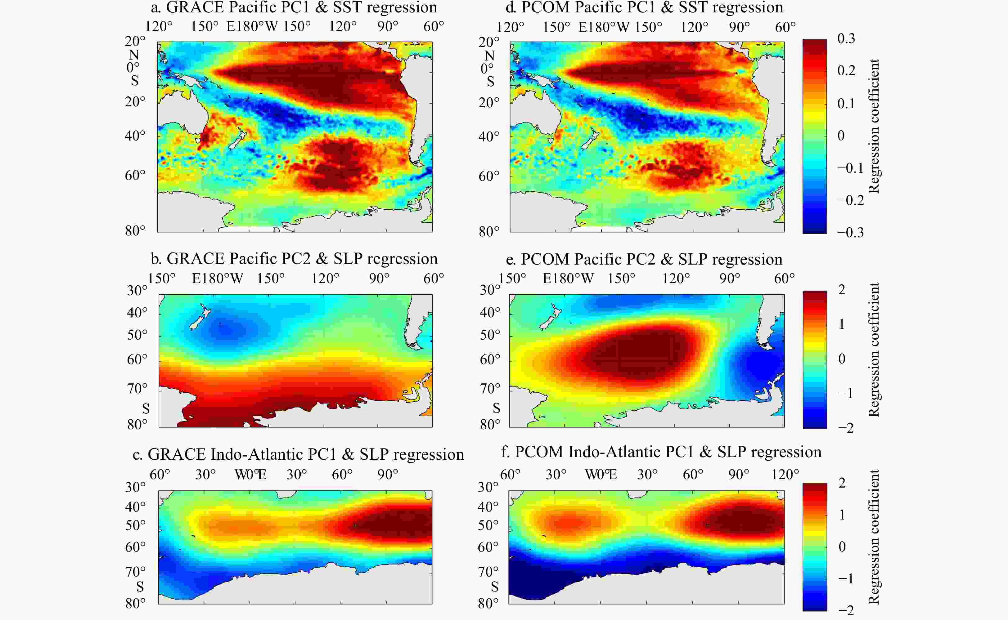
Figure 9. SST (unit: °C) pattern regressed onto PC1 time series (upper panels) and SLP (unit: hPa) pattern regressed onto PC2 time series (middle panels) in the South Pacific Ocean, and SLP pattern regressed onto PC1 time series of OBP anomaly in the South Indo-Atlantic Ocean (lower panels); OBP based on GRACE (left panels) and PCOM (right panels). The anomalies are calculated by subtracting climatological annual cycle.

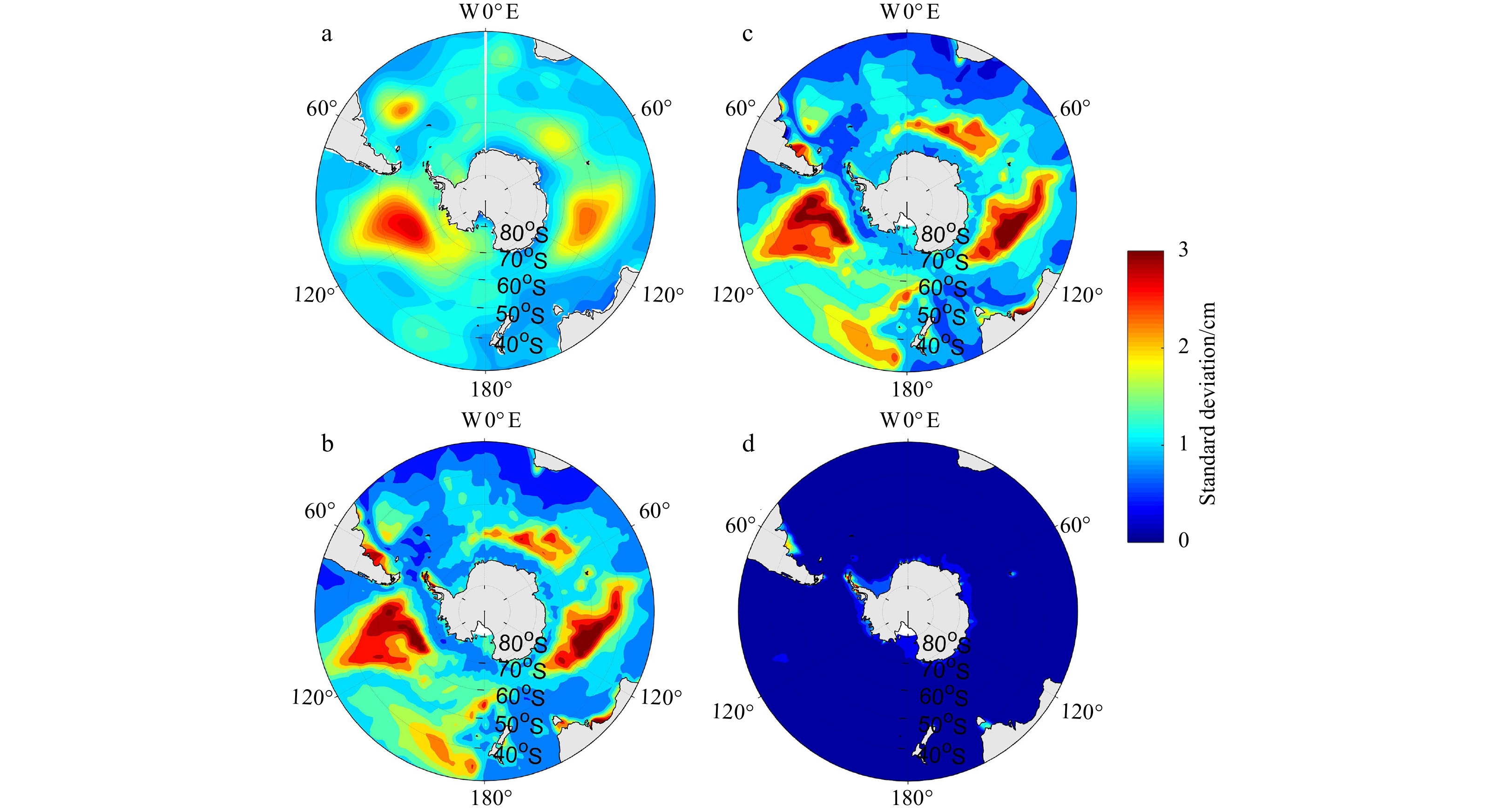
Figure 10. Standard deviation of interannual GRACE OBP (in unit of cm) in the Southern Ocean (a), standard deviation of interannual OBP in the Southern Ocean from control run of PCOM (Exp. 1) (b), standard deviation of interannual OBP in the Southern Ocean from control run of PCOM (Exp. 2) (c), and standard deviation of interannual OBP in the Southern Ocean from control run of PCOM (Exp. 3) (d) from 2003 to 2016.

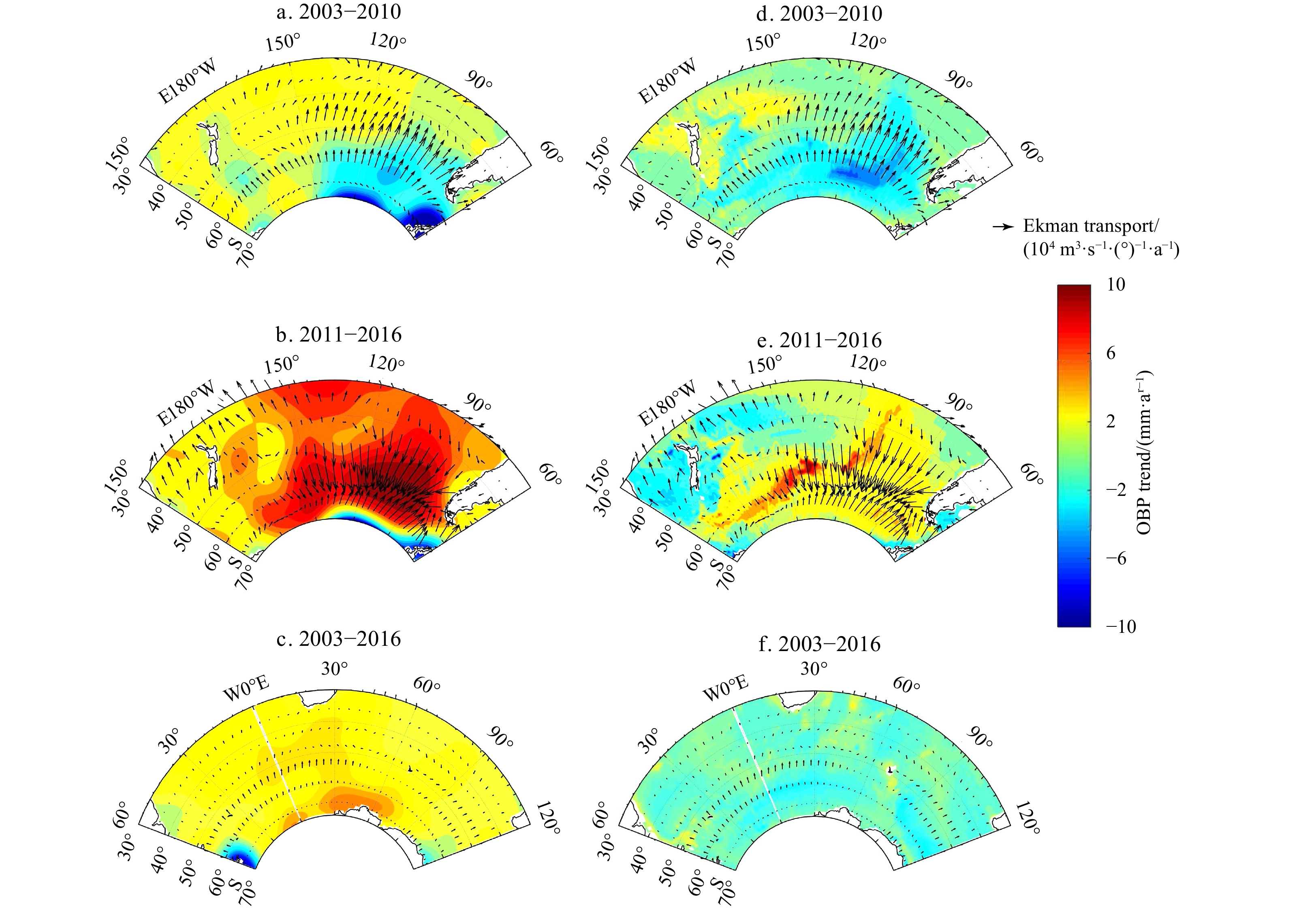
Figure 11. Trends of OBP (color shading, mm/a) and Ekman transport (vector, m3/(°)) based on Grace (left panels) and PCOM (right panels). a, b, d and e. For the two periods of 2003–2010 (a, d) and 2011–2016 (b, e) in the South Pacific Ocean; c and f. for the period of 2003–2016 in the South Indo-Atlantic Ocean.
-
[1] Androsov A, Boebel O, Schröter J, et al. 2020. Ocean bottom pressure variability: Can it be reliably modeled?. Journal of Geophysical Research: Oceans, 125(3): e2019JC015469 [2] Antonov J I, Seidov D, Boyer T P, et al. 2010. World Ocean Atlas 2009, Volume 2: Salinity. NOAA Atlas NESDIS 69. Washington, DC: U S Government Printing Office [3] Bergmann I, Dobslaw H. 2012. Short-term transport variability of the Antarctic Circumpolar Current from satellite gravity observations. Journal of Geophysical Research: Oceans, 117(C5): C05044 [4] Boening C, Lee T, Zlotnicki V. 2011. A record-high ocean bottom pressure in the South Pacific observed by GRACE. Geophysical Research Letters, 38(4): L04602 [5] Boening C, Willis J K, Landerer F W, et al. 2012. The 2011 La Niña: So strong, the oceans fell. Geophysical Research Letters, 39(19): L19602 [6] Brunnabend S E, Rietbroek R, Timmermann R, et al. 2011. Improving mass redistribution estimates by modeling ocean bottom pressure uncertainties. Journal of Geophysical Research: Oceans, 116(C8): C08037 [7] Cabanes C, Huck T, De Verdière A C. 2006. Contributions of wind forcing and surface heating to interannual sea level variations in the Atlantic Ocean. Journal of Physical Oceanography, 36(9): 1739–1750 doi: 10.1175/JPO2935.1 [8] Cazenave A, Dieng H B, Meyssignac B, et al. 2014. The rate of sea-level rise. Nature Climate Change, 4(5): 358–361 doi: 10.1038/nclimate2159 [9] Cazenave A, Henry O, Munier S, et al. 2012. Estimating ENSO influence on the global mean sea level, 1993–2010. Marine Geodesy, 35(S1): 82–97 [10] Chambers D P, Cazenave A, Champollion N, et al. 2017. Evaluation of the global mean sea level budget between 1993 and 2014. Surveys in Geophysics, 38(1): 309–327 doi: 10.1007/s10712-016-9381-3 [11] Cheng Xuhua, Li Lijuan, Du Yan, et al. 2013. Mass-induced sea level change in the northwestern North Pacific and its contribution to total sea level change. Geophysical Research Letters, 40(15): 3975–3980 doi: 10.1002/grl.50748 [12] Dukowicz J K. 1997. Steric sea level in the los alamos POP code—non-boussinesq effects. Atmosphere-Ocean, 35(S1): 533–546 [13] Fasullo J T, Boening C, Landerer F W, et al. 2013. Australia's unique influence on global sea level in 2010–2011. Geophysical Research Letters, 40(16): 4368–4373 doi: 10.1002/grl.50834 [14] Gill A E, Niller P P. 1973. The theory of the seasonal variability in the ocean. Deep Sea Research and Oceanographic Abstracts, 20(2): 141–177 doi: 10.1016/0011-7471(73)90049-1 [15] Greatbatch R J. 1994. A note on the representation of steric sea level in models that conserve volume rather than mass. Journal of Geophysical Research: Oceans, 99(C6): 12767–12771 doi: 10.1029/94JC00847 [16] Henley B J, Gergis J, Karoly D J, et al. 2015. A tripole index for the interdecadal Pacific oscillation. Climate Dynamics, 45(11–12): 3077–3090 doi: 10.1007/s00382-015-2525-1 [17] Huang Ruixin, Jin Xiangze, Zhang Xuehong. 2001. An oceanic general circulation model in pressure coordinates. Advances in Atmospheric Sciences, 18(1): 1–22 doi: 10.1007/s00376-001-0001-9 [18] Johnson G C, Chambers D P. 2013. Ocean bottom pressure seasonal cycles and decadal trends from GRACE Release-05: Ocean circulation implications. Journal of Geophysical Research: Oceans, 118(9): 4228–4240 doi: 10.1002/jgrc.20307 [19] Kalnay E, Kanamitsu M, Kistler R, et al. 1996. The NCEP/NCAR 40-year reanalysis project. Bulletin of the American Meteorological Society, 77(3): 437–472 doi: 10.1175/1520-0477(1996)077<0437:TNYRP>2.0.CO;2 [20] Li Hong, Xu Fanghua, Zhou Wei, et al. 2017. Development of a global gridded Argo data set with Barnes successive corrections. Journal of Geophysical Research: Oceans, 122(2): 866–889 doi: 10.1002/2016JC012285 [21] Liau J R, Chao B F. 2017. Variation of Antarctic circumpolar current and its intensification in relation to the southern annular mode detected in the time-variable gravity signals by GRACE satellite. Earth, Planets and Space, 69: 93 [22] Locarnini R A, Mishonov A V, Antonov J I, et al. 2010. World Ocean Atlas 2009, Volume 1: Temperature. NOAA Atlas NESDIS 68. Washington, DC: U S Government Printing Office [23] Makowski J K, Chambers D P, Bonin J A. 2015. Using ocean bottom pressure from the gravity recovery and climate experiment (GRACE) to estimate transport variability in the southern Indian Ocean. Journal of Geophysical Research: Oceans, 120(6): 4245–4259 doi: 10.1002/2014JC010575 [24] Marshall G J. 2003. Trends in the southern annular mode from observations and reanalyses. Journal of Climate, 16(24): 4134–4143 doi: 10.1175/1520-0442(2003)016<4134:TITSAM>2.0.CO;2 [25] Meredith M P, Woodworth P L, Chereskin T K, et al. 2011. Sustained monitoring of the southern ocean at drake passage: Past achievements and future priorities. Reviews of Geophysics, 49(4): RG4005 [26] Ou Niansen, Lin Yihua, Bi Xunqiang, et al. 2016. Baseline evaluation of a pressure coordinate ocean model (PCOM 1.0). Climatic and Environmental Research (in Chinese), 21(1): 56–64 [27] Peralta-Ferriz C, Landerer F W, Chambers D, et al. 2017. Remote sensing of bottom pressure from GRACE satellites. US CLIVAR Variations Newsletter, 15(2): 22–28 [28] [29] Piecuch C G, Quinn K J, Ponte R M. 2013. Satellite-derived interannual ocean bottom pressure variability and its relation to sea level. Geophysical Research Letters, 40(12): 3106–3110 doi: 10.1002/grl.50549 [30] Ponte R M. 1999. A preliminary model study of the large-scale seasonal cycle in bottom pressure over the global ocean. Journal of Geophysical Research: Oceans, 104(C1): 1289–1300 doi: 10.1029/1998JC900028 [31] Ponte R M, Piecuch C G. 2014. Interannual bottom pressure signals in the Australian–Antarctic and Bellingshausen basins. Journal of Physical Oceanography, 44(5): 1456–1465 doi: 10.1175/JPO-D-13-0223.1 [32] Quinn K J, Ponte R M. 2012. High frequency barotropic ocean variability observed by GRACE and satellite altimetry. Geophysical Research Letters, 39(7): L07603 [33] Song Y T, Zlotnicki V. 2008. Subpolar ocean bottom pressure oscillation and its links to the tropical ENSO. International Journal of Remote Sensing, 29(21): 6091–6107 doi: 10.1080/01431160802175538 [34] Stammer D, Tokmakian R, Semtner A, et al. 1996. How well does a 1/4° global circulation model simulate large-scale oceanic observations?. Journal of Geophysical Research: Oceans, 101(C11): 25779–25811 [35] Stepanov V N, Hughes C W. 2006. Propagation of signals in basin-scale ocean bottom pressure from a barotropic model. Journal of Geophysical Research: Oceans, 111(C12): C12002 doi: 10.1029/2005JC003450 [36] Thomson R E, Tabata S. 1989. Steric sea level trends in the northeast Pacific Ocean: Possible evidence of global sea level rise. Journal of Climate, 2(6): 542–553 doi: 10.1175/1520-0442(1989)002<0542:SSLTIT>2.0.CO;2 [37] Vivier F, Kelly K A, Harismendy M. 2005. Causes of large-scale sea level variations in the Southern Ocean: Analyses of sea level and a barotropic model. Journal of Geophysical Research: Oceans, 110(C9): C09014 [38] Wang Juan, Wang Jing, Cheng Xuhua. 2015. Mass-induced sea level variations in the Gulf of Carpentaria. Journal of Oceanography, 71(4): 449–461 doi: 10.1007/s10872-015-0304-6 [39] Zhang Yu, Lin Yihua, Huang Ruixin. 2014. A climatic dataset of ocean vertical turbulent mixing coefficient based on real energy sources. Science China Earth Sciences, 57(10): 2435–2446 doi: 10.1007/s11430-014-4904-6 [40] Zlotnicki V, Wahr J, Fukumori I, et al. 2007. Antarctic circumpolar current transport variability during 2003–05 from GRACE. Journal of Physical Oceanography, 37(2): 230–244 doi: 10.1175/JPO3009.1 -

 下载:
下载:


 点击查看大图

计量
- 文章访问数: 478
- HTML全文浏览量: 143
- PDF下载量: 29
- 被引次数: 0