

Intra-seasonal variability of the abyssal currents in COMRA’s contract area in the Clarion-Clipperton Zone
-
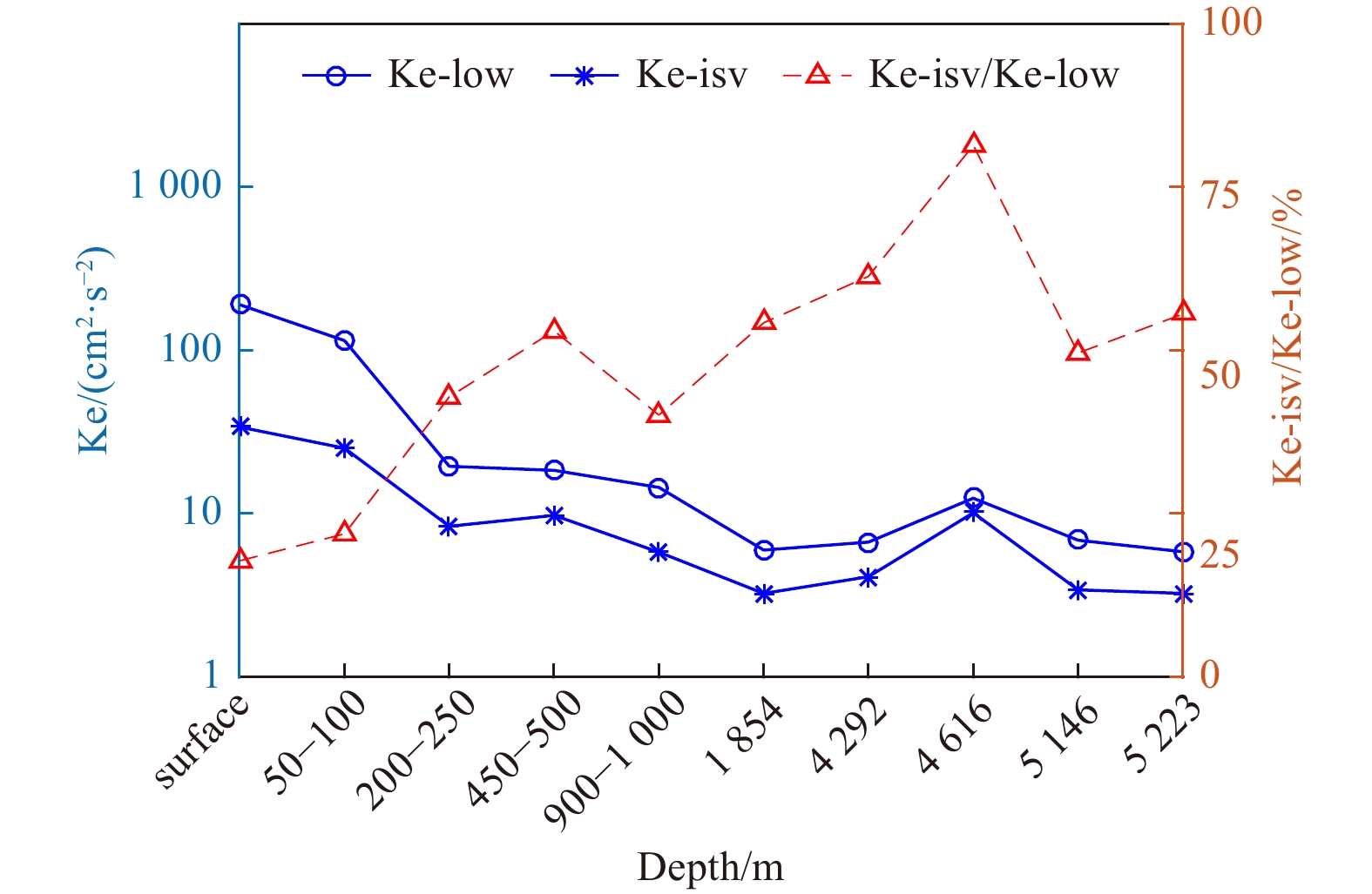
Abstract: In this paper, the intra-seasonal variability of the abyssal currents in the China Ocean Mineral Resources Association (COMRA) polymetallic nodule contact area, located in the western part of the Clarion and Clipperton Fraction Zone in the tropical East Pacific, is investigated using direct observations from subsurface mooring instruments as well as sea-surface height data and reanalysis products. Mooring observations were conducted from September 13, 2017 to August 15, 2018 in the COMRA contact area (10°N, 154°W). The results were as follows: (1) At depths below 200 m, the kinetic energy of intra-seasonal variability (20−100 d) accounts for more than 40% of the overall low-frequency variability, while the ratio reaches more than 50% below 2 000 m. (2) At depths below 200 m, currents show a synchronous oscillation with a characteristic time scale of 30 d, lasting from October to the following January; the energy of the 30-d oscillation increases with depth until the layer of approximately 4 616 m, and the maximum velocity is approximately 10 cm/s. (3) The 30-d oscillation of deep currents is correlated with the tropical instability waves in the upper ocean.
-
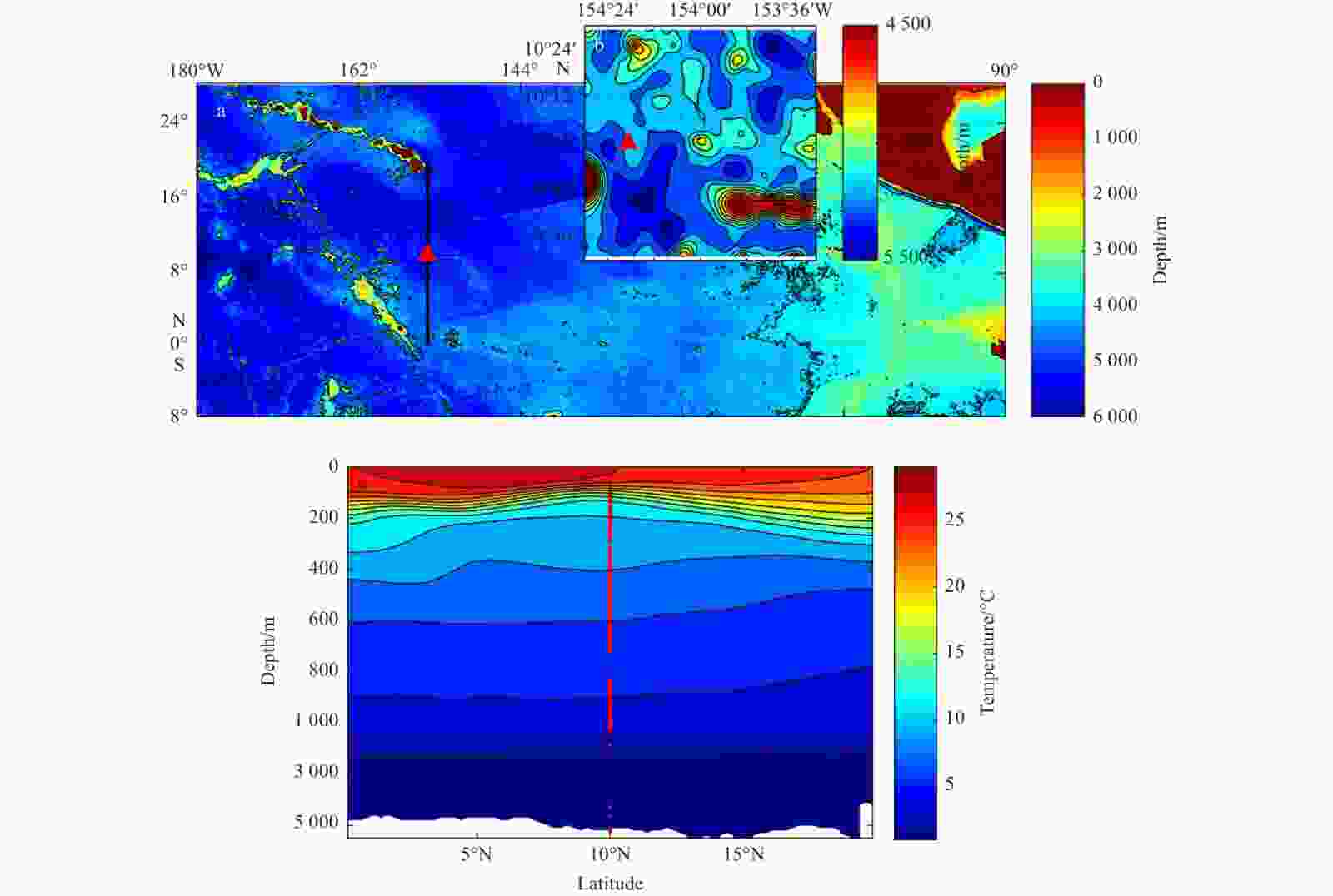
Figure 1. ETOPO1 depth of the eastern tropical Pacific Ocean, position of the mooring site (red triangle) and the section in c (a); depth around the mooring site (b); climatologic temperature (from World Ocean Atlas 2009) at a meridional section of 154°W (0°−20°N) and the observation range of current metres (red line represents the observation range of 75-kHz ADCPs at upper layers and the red dots below 1 200 m represent the location of Aquadopp current meters) (c).
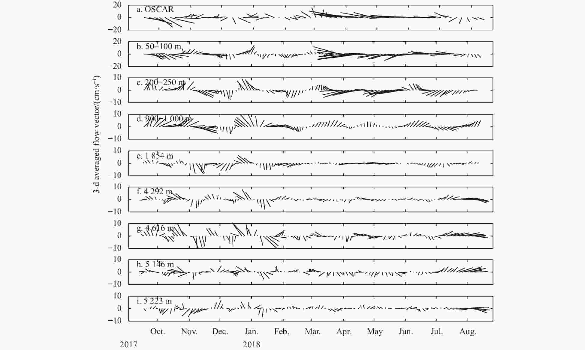
Figure 2. Time series of 3-d averaged flow vectors after 3-d low-pass filtering at different depths.
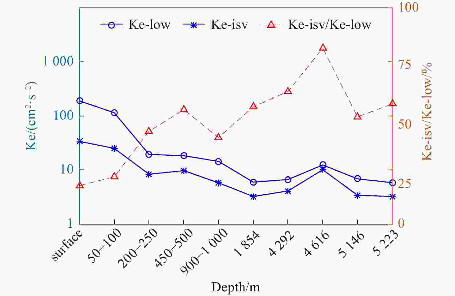
Figure 3. Kinetic energy of intra-seasonal variability (ISV), low-frequency variability and their ratio. The blue circle line represents kinetic energy of low-frequency variability (Ke-low); the blue asterick line represents kinetic energy of ISV (Ke-isv); the red triangle line represents the ratio of Ke-isv and Ke-low.

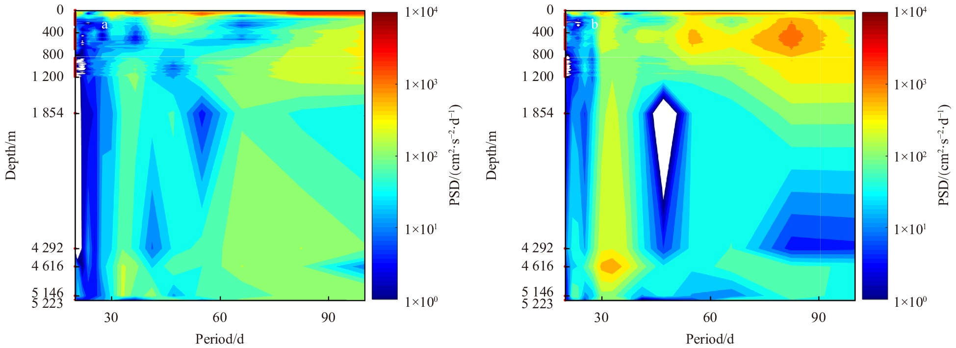
Figure 4. Power spectral density (PSD) of the velocity in zonal (a) and meridional (b) currents.
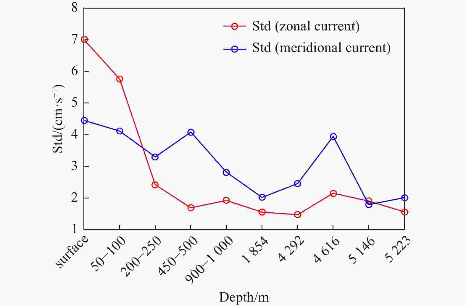
Figure 5. Standard deviations (Std) of the meridional and zonal velocities at the intra-seasonal time scale.
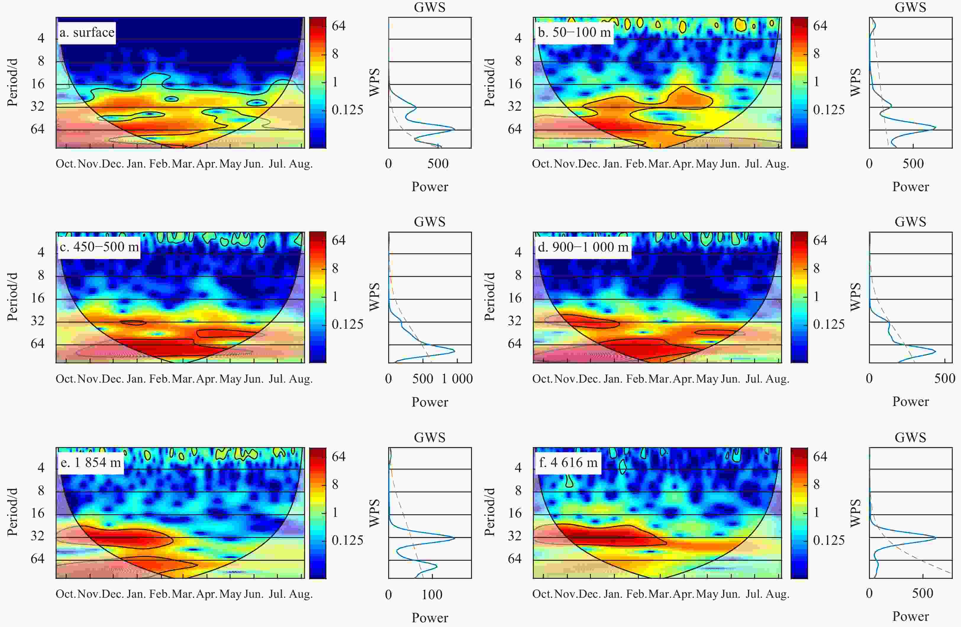
Figure 6. Continuous wavelet transform of meridional velocity at surface current (a) and currents at 50−100 m (b), 450−500 m (c), 900−1 000 m (d), 1 854 m (e) , 4 616 m (f). The colour filled maps represent the wavelet power spectrum (WPS), and the curves on the right represent the global wavelet spectrum (GWS). In the colour maps, the thick black contours denote the 5% significance level against red noise. The cone of influence where edge effects might distort the picture is shown in lighter shades.
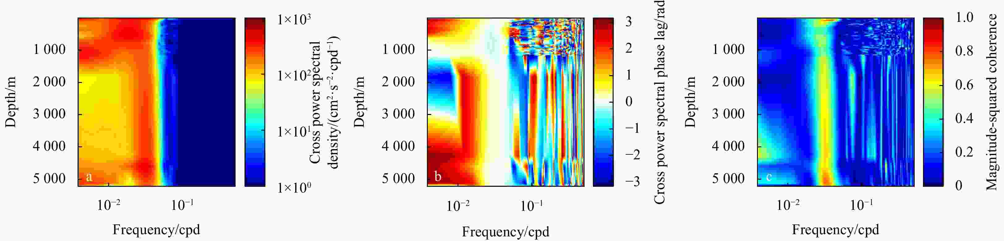
Figure 7. Cross spectrum analysis between the surface meridional current (OSCAR) and those at other depths. a. Cross power spectral density; b. cross power spectral phase lag; c. magnitude-squared coherence. The cpd means counts per day.
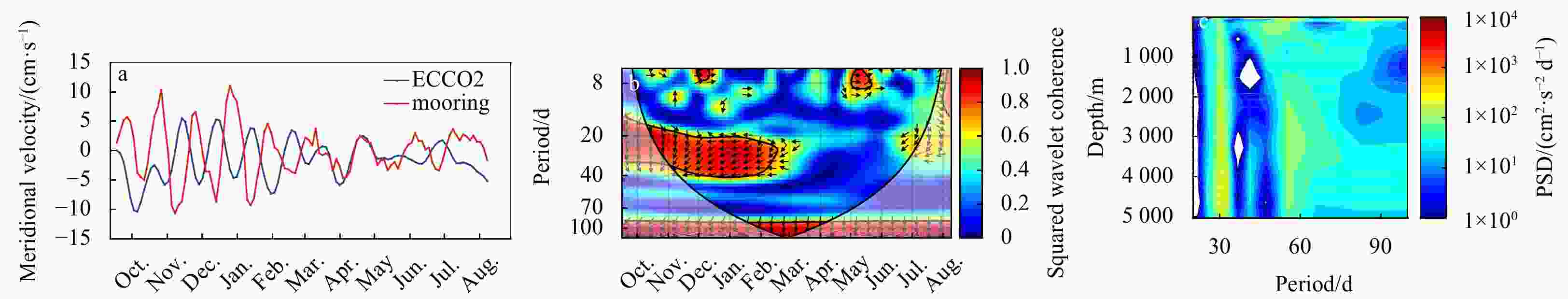
Figure 9. Comparison of meridional velocity at 4 616 m from observations and reanalysis products. a. Time series; b. squared wavelet coherence; c. power spectral density (PSD) of the meridional velocity at the mooring site, from reanalysis data.

Figure 10. Spatial amplitude (a), spatial phase (b), spatial reconstruction (c), temporal amplitude (d), temporal phase (e), frequency-spectra density (f) of the first complex empirical orthogonal function (CEOF) mode of meridional velocity at 4 000 m. The mooring site is marked with a triangle in a, b and c. The cpd means counts per day.
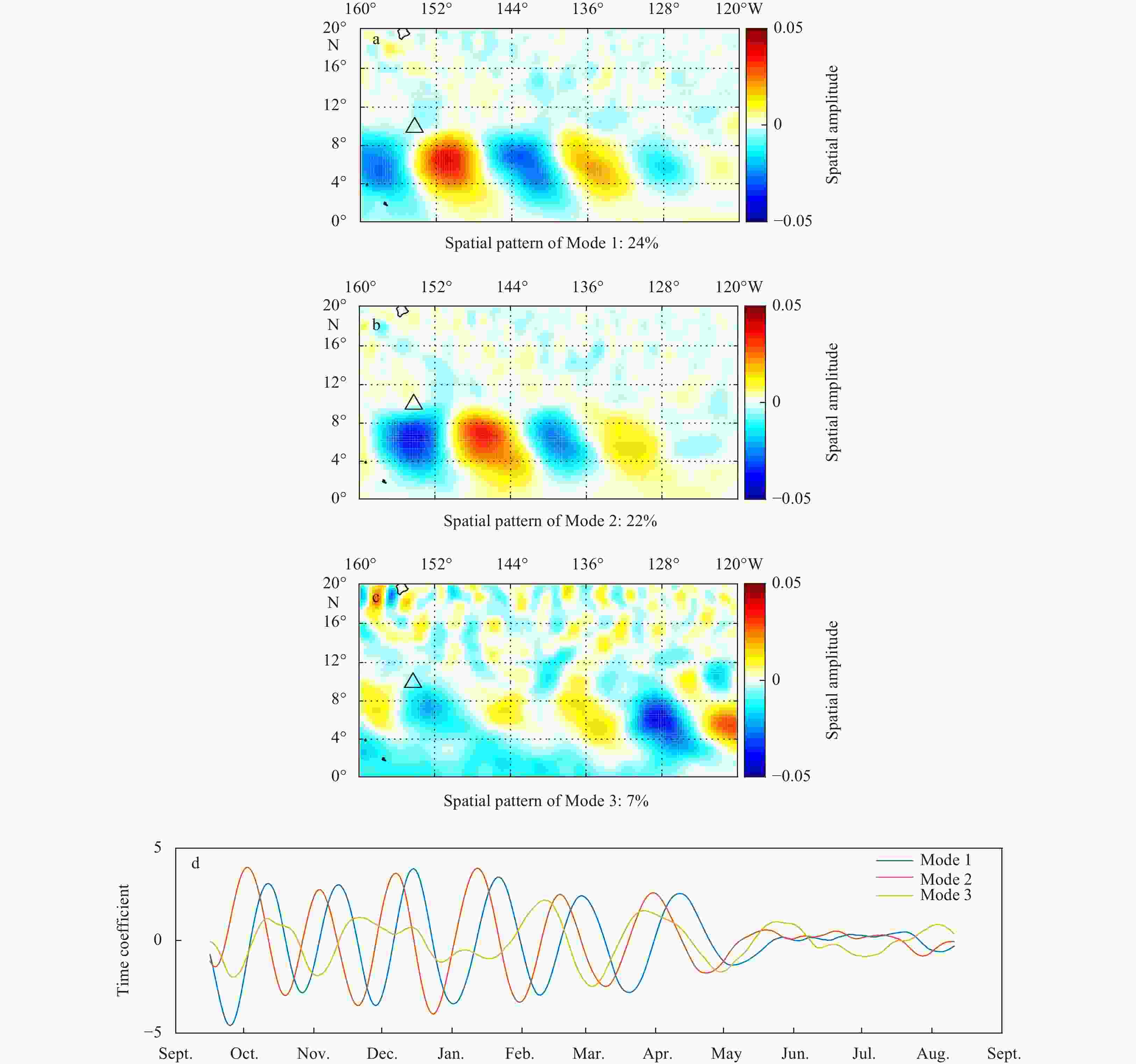
Figure 11. The first three empirical orthogonal function modes of sea level anomaly at the intra-seasonal time scale.

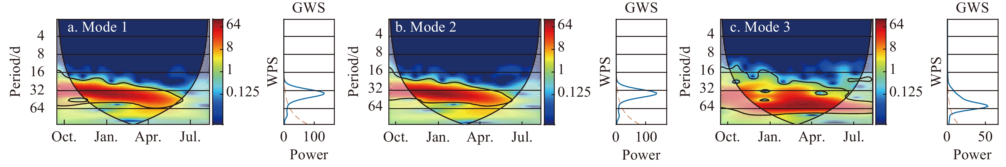
Figure 12. Continuous wavelet transform of the time series of the first three empirical orthogonal function modes of sea level anomaly. WPS: wavelet power spectrum; GWS: global wavelet spectrum.
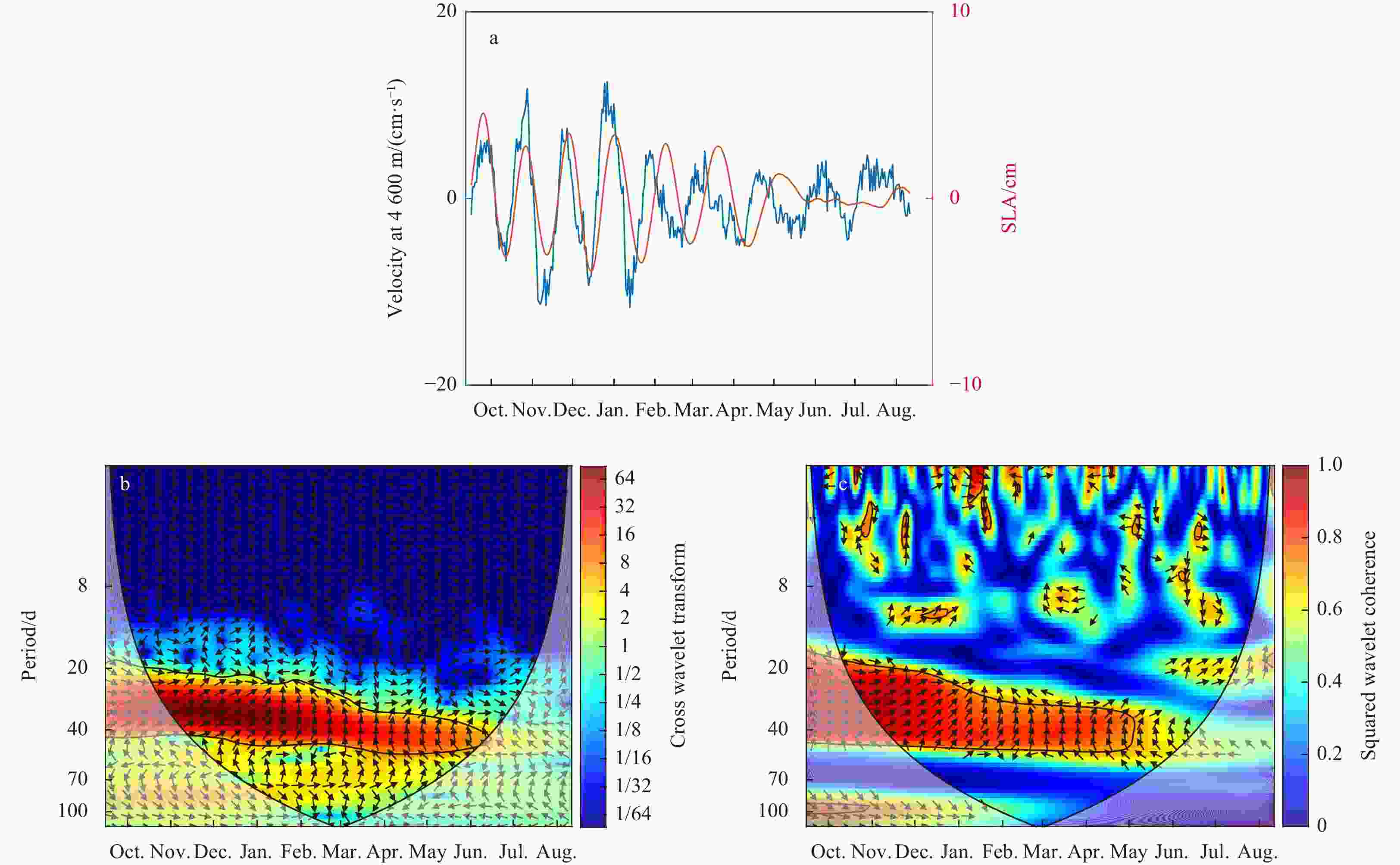
Figure 13. Time series of the first empirical orthogonal function (EOF) mode of sea level anomaly (SLA) and meridional velocity at 4 616 m (a); cross wavelet transform (b) and squared wavelet coherence (c) between the time series of the first EOF mode of SLA and meridional velocity at 4 616 m.
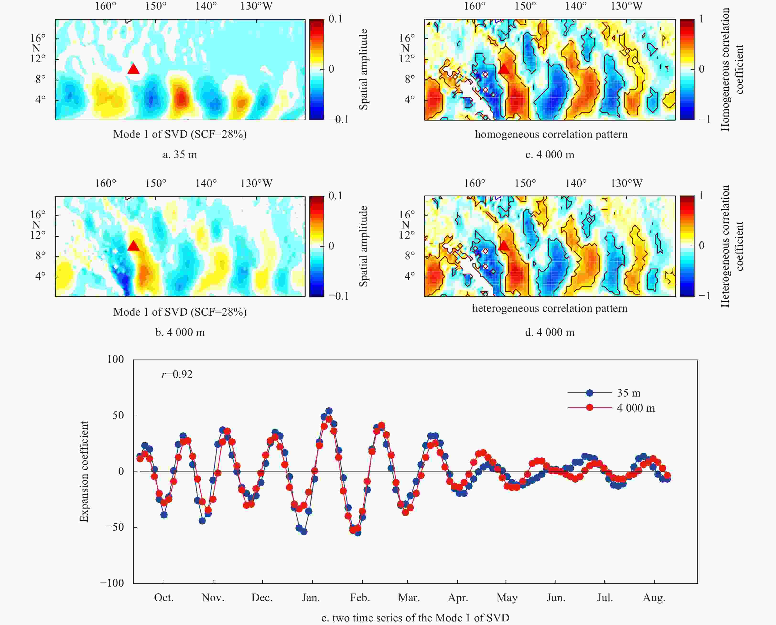
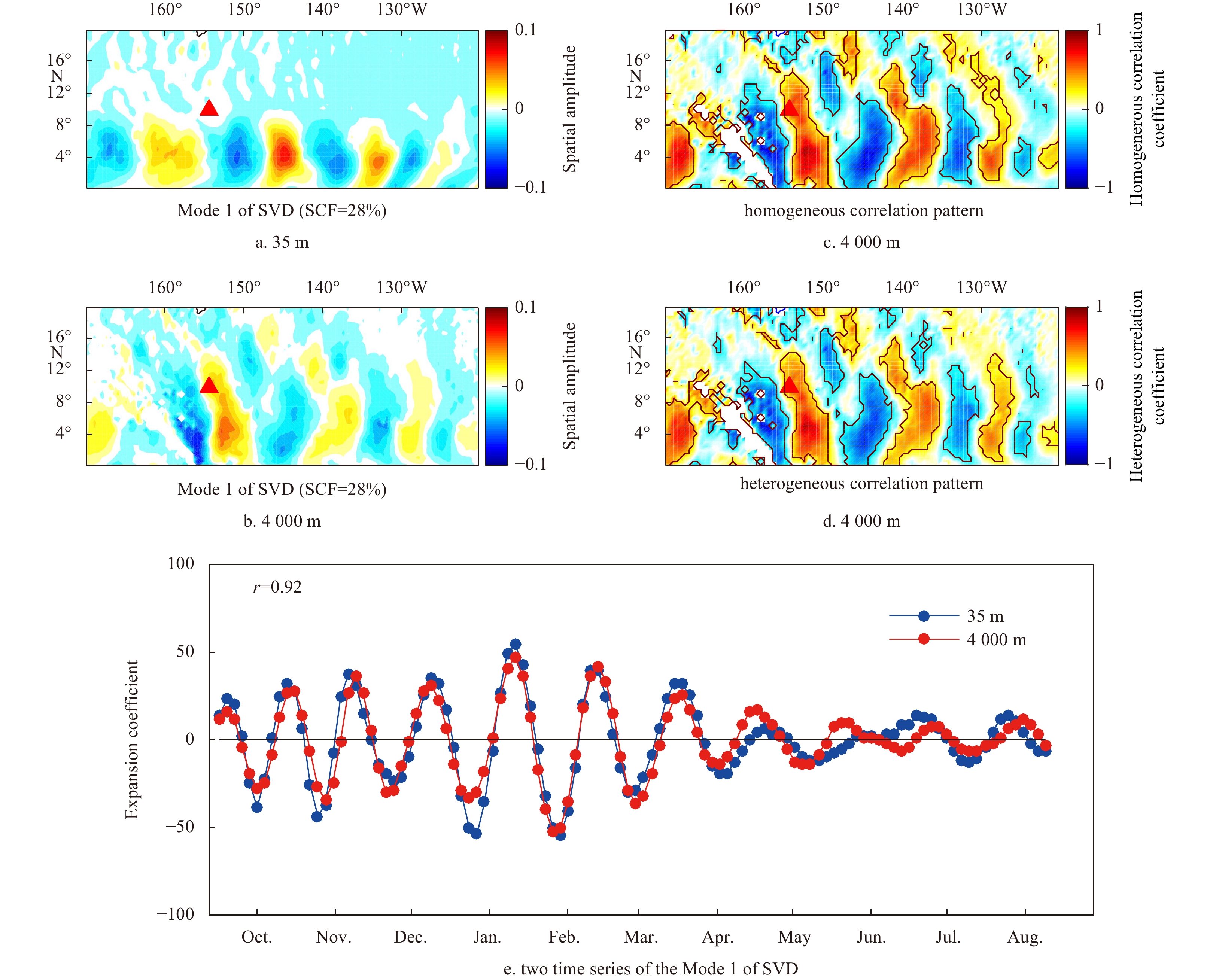
Figure 14. Spatial patterns of 35 m (a) and 4 000 m (b) meridional velocity; homogeneous (c) and heterogeneous (d) correlation map for the 4 000 m velocity, the 95% significance level is shown as red contours; time evolution of the expansion coefficients of 35 m and 4 000 m meridional velocity (e). All is for the first leading SVD mode. The mooring site is marked with a red triangle in a and b. SVD: Singular Value Decomposition; SCF: Squared Covariance Fraction (measuring the amount of squared covariance for which each mode accounts).
-
Aleynik D, Inall M E, Dale A, et al. 2017. Impact of remotely generated eddies on plume dispersion at abyssal mining sites in the Pacific. Scientific Reports, 7(1): 16959. doi: 10.1038/s41598-017-16912-2 Cox M D. 1980. Generation and propagation of 30-Day waves in a numerical model of the Pacific. Journal of Physical Oceanography, 10(8): 1168–1186. doi: 10.1175/1520-0485(1980)010<1168:GAPODW>2.0.CO;2 Enfield D B. 1987. The intraseasonal oscillation in eastern Pacific sea levels: how is it forced?. Journal of Physical Oceanography, 17(11): 1860–1876. doi: 10.1175/1520-0485(1987)017<1860:TIOIEP>2.0.CO;2 Eriksen C C. 1985. Moored observations of deep Low-Frequency motions in the central Pacific Ocean: vertical structure and interpretation as equatorial waves. Journal of Physical Oceanography, 15(8): 1085–1113. doi: 10.1175/1520-0485(1985)015<1085:MOODLF>2.0.CO;2 Eriksen C C, Richman J. 1988. An estimate of equatorial wave energy flux at 9- to 90-day periods in the Central Pacific. Journal of Geophysical Research: Oceans, 93(C12): 15455–15466. doi: 10.1029/JC093iC12p15455 Farrar J T. 2011. Barotropic Rossby waves radiating from tropical instability waves in the Pacific Ocean. Journal of Physical Oceanography, 41(6): 1160–1181. doi: 10.1175/2011JPO4547.1 Hamilton P. 2009. Topographic Rossby waves in the Gulf of Mexico. Progress in Oceanography, 82(1): 1–31. doi: 10.1016/j.pocean.2009.04.019 Hamilton P, Bower A, Furey H, et al. 2019. The loop current: observations of deep eddies and topographic waves. Journal of Physical Oceanography, 49(6): 1463–1483. doi: 10.1175/JPO-D-18-0213.1 Liang Xinfeng, Thurnherr A M. 2011. Subinertial variability in the deep ocean near the East Pacific Rise between 9° and 10°N. Geophysical Research Letters, 38(6): L06606 Liu Qinyu, Pan Aijun, Liu Zhengyu. 2003. Intraseasonal oscillation and baroclinic instability of upper layer ocean in the north equator current. Oceanologia et Limnologia Sinica, 34(1): 94–100 Liu Yansong, Yu Fei, Nan Feng, et al. 2019. Intraseasonal oscillation of deep currents influenced by mesoscale eddies in the Kuroshio Extension Region. Scientific Reports, 9(1): 4147. doi: 10.1038/s41598-019-39567-7 Ma Qiang, Wang Fan, Wang Jianing, et al. 2019. Intensified deep ocean variability induced by topographic rossby waves at the Pacific Yap-Mariana junction. Journal of Geophysical Research: Oceans, 124(11): 8360–8374. doi: 10.1029/2019JC015490 Menemenlis D, Fukumori I, Lee T. 2005. Using green’s functions to calibrate an ocean general circulation model. Monthly Weather Review, 133(5): 1224–1240. doi: 10.1175/MWR2912.1 Oey L Y. 2008. Loop current and deep eddies. Journal of Physical Oceanography, 38(7): 1426–1449. doi: 10.1175/2007JPO3818.1 Oey L Y, Lee H C. 2002. Deep eddy energy and topographic Rossby waves in the Gulf of Mexico. Journal of Physical Oceanography, 32(12): 3499–3527. doi: 10.1175/1520-0485(2002)032<3499:DEEATR>2.0.CO;2 Qiao Fangli, Tal E, Yuan Yeli. 2004. The zonal distribution features of high frequency oscillations in the oceans derived from satellite altimeter data. Haiyang Xuebao (in Chinese), 26(3): 1–7 Qiao L, Weisberg R H. 1995. Tropical instability wave kinematics: observations from the Tropical Instability Wave Experiment. Journal of Geophysical Research: Oceans, 100(C5): 8677–8693. doi: 10.1029/95JC00305 Shu Yeqiang, Xue Huijie, Wang Dongxiao, et al. 2016. Persistent and energetic bottom-trapped topographic Rossby waves observed in the southern South China Sea. Scientific Reports, 6(1): 24338. doi: 10.1038/srep24338 Spillane M C, Enfield D B, Allen J S. 1987. Intraseasonal oscillations in sea level along the west coast of the Americas. Journal of Physical Oceanography, 17(3): 313–325. doi: 10.1175/1520-0485(1987)017<0313:IOISLA>2.0.CO;2 Sun Jilin, Li Li. 1998. Priliminary analysis on Lower Frequency Waves in the Equatorial Pacific. Journal of Ocean University of Qingdao, (3): 24–30 Wang Fujun, Zhang Linlin, Hu Dunxin, et al. 2017. The vertical structure and variability of the western boundary currents east of the Philippines: case study from in situ observations from December 2010 to August 2014. Journal of Oceanography, 73(6): 743–758. doi: 10.1007/s10872-017-0429-x Willett C S, Leben R R, Lavín M F. 2006. Eddies and Tropical Instability Waves in the eastern tropical Pacific: a review. Progress in Oceanography, 69(1–2): 218–238 Yoshioka N, Endoh M, Ishizaki H. 1988. Observation of the abyssal current in the West Mariana Basin. Journal of the Oceanographical Society of Japan, 44(1): 33–39. doi: 10.1007/BF02303148 Zhai Ping. 2008. The distribution characteristic and mechanism of intraseasonal oscillations in global oceans (in Chinese) [dissertation]. Qingdao: Ocean University of China Zhu Yingli, Liang Xinfeng. 2020. Coupling of the surface and Near-Bottom currents in the Gulf of Mexico. Journal of Geophysical Research: Oceans, 125(11): e2020JC016488 -

 下载:
下载:


 点击查看大图

计量
- 文章访问数: 525
- HTML全文浏览量: 173
- PDF下载量: 38
- 被引次数: 0