

Objective array design for three-dimensional temperature and salinity observation: Application to the South China Sea
-
Abstract: In this study, a moored array optimization tool (MAOT) was developed and applied to the South China Sea (SCS) with a focus on three-dimensional temperature and salinity observations. Application of the MAOT involves two steps: (1) deriving a set of optimal arrays that are independent of each other for different variables at different depths based on an empirical orthogonal function method, and (2) consolidating these arrays using a K-center clustering algorithm. Compared with the assumed initial array consisting of 17 mooring sites located on a 3°×3° horizontal grid, the consolidated array improved the observing ability for three-dimensional temperature and salinity in the SCS with optimization efficiencies of 19.03% and 21.38%, respectively. Experiments with an increased number of moored sites showed that the most cost-effective option is a total of 20 moorings, improving the observing ability with optimization efficiencies up to 26.54% for temperature and 27.25% for salinity. The design of an objective array relies on the ocean phenomenon of interest and its spatial and temporal scales. In this study, we focus on basin-scale variations in temperature and salinity in the SCS, and thus our consolidated array may not well resolve mesoscale processes. The MAOT can be extended to include other variables and multi-scale variability and can be applied to other regions.
-
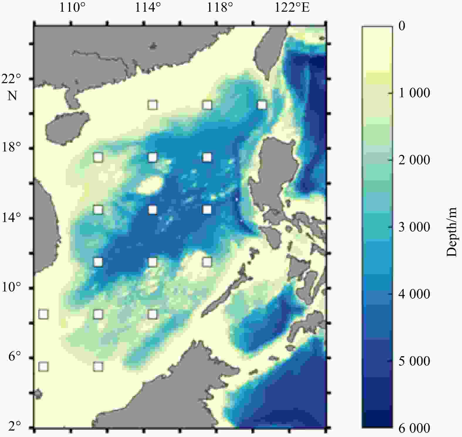
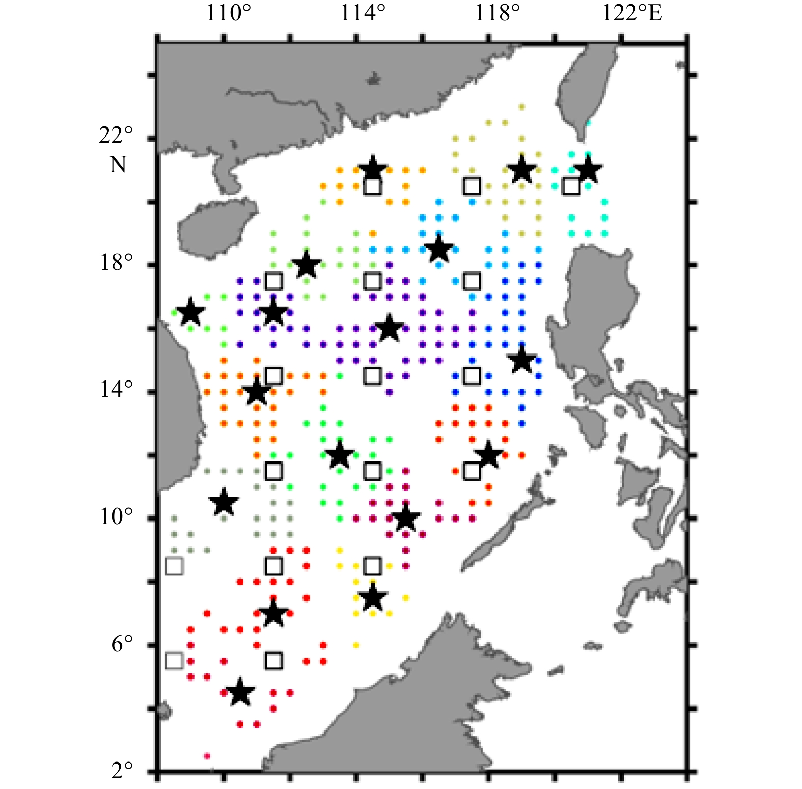
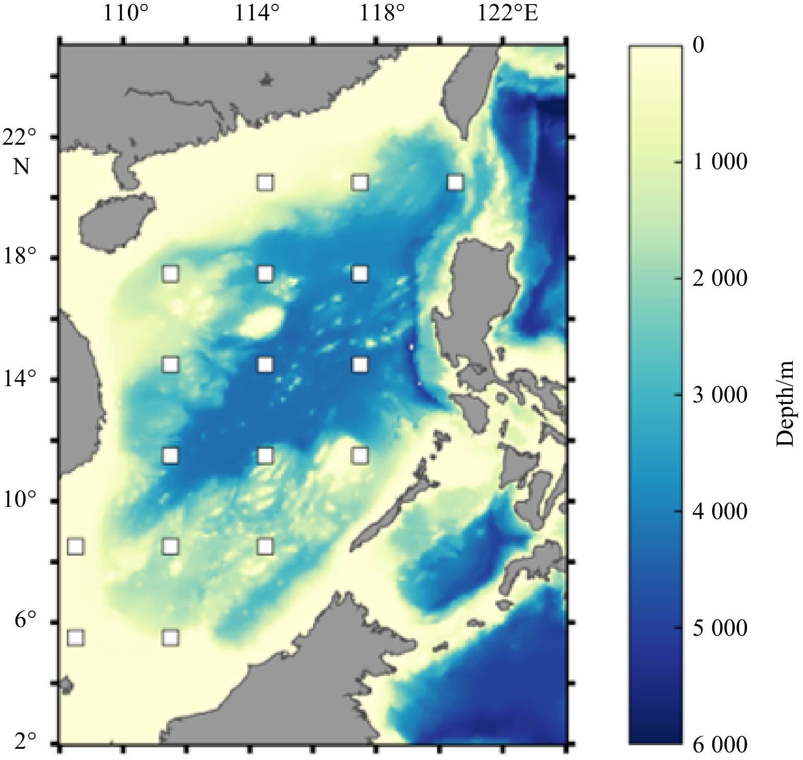
Figure 1. Topography of the South China Sea. White squares represent the locations of the assumed initial array.
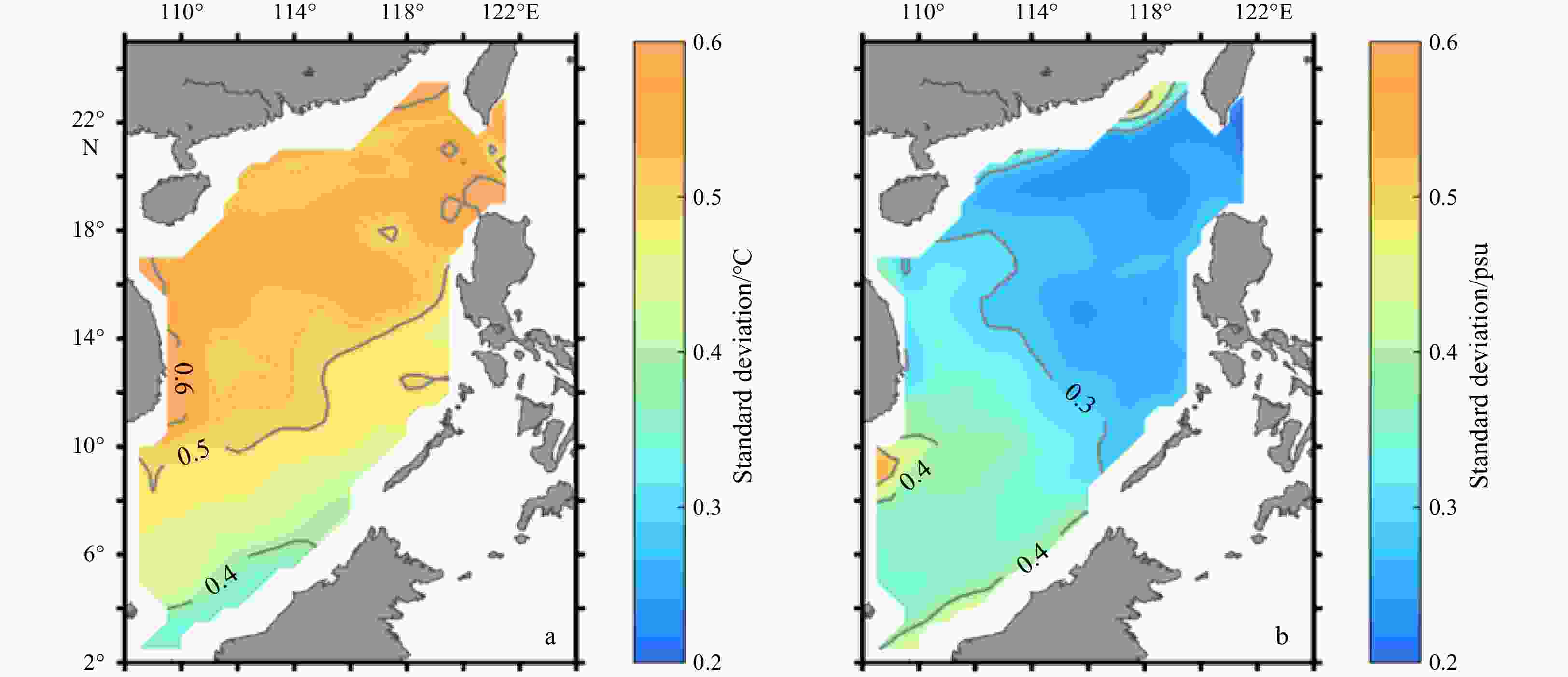
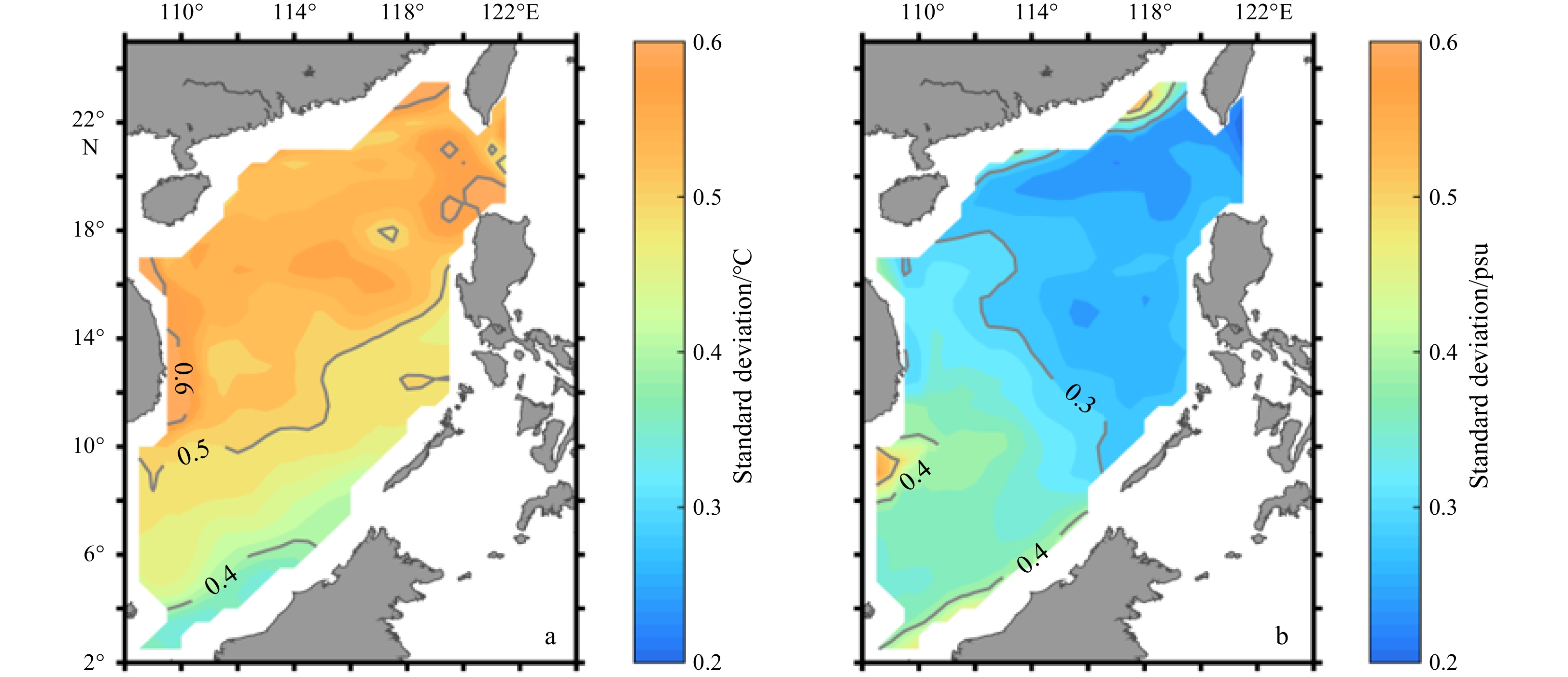
Figure 2. Standard deviation of sea surface temperature (a) and salinity anomalies (b).

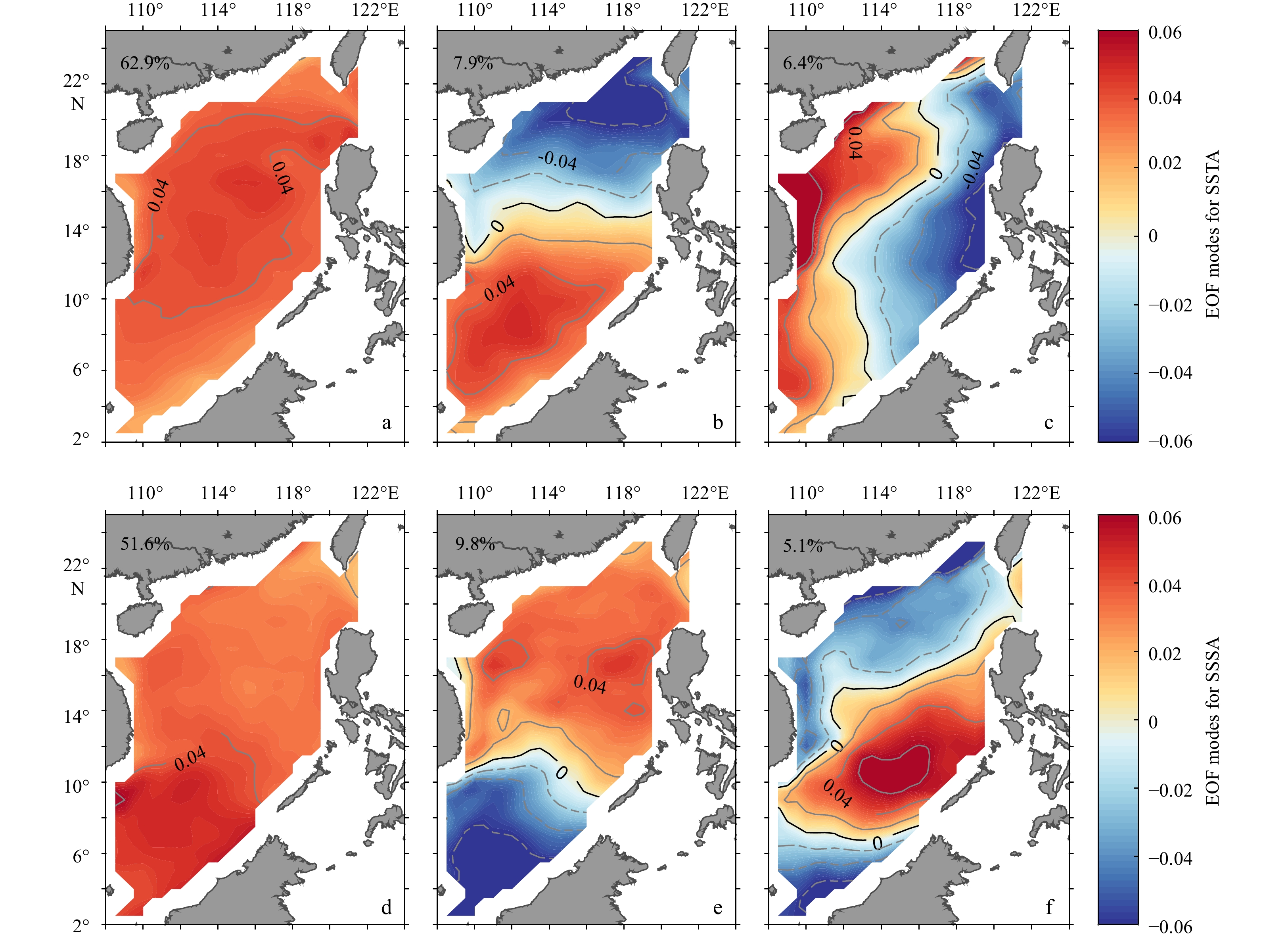
Figure 3. Spatial patterns of the first (a), second (b), and third (c) empirical orthogonal function (EOF) modes for sea surface tem-perature anomalies (SSTA) in the South China Sea; d–f are the same as a–c but for sea surface salinity anomalies (SSSA).
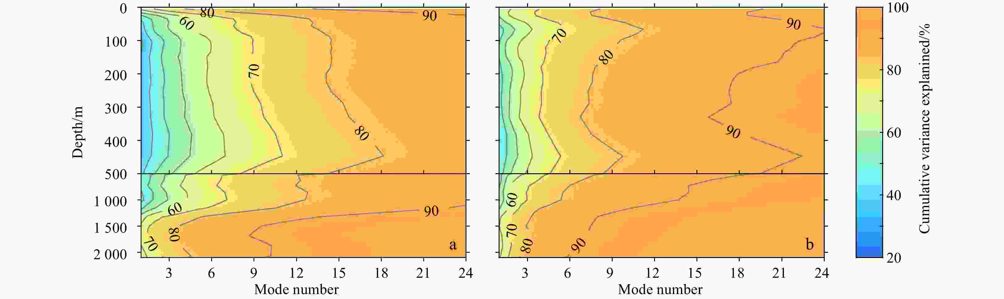
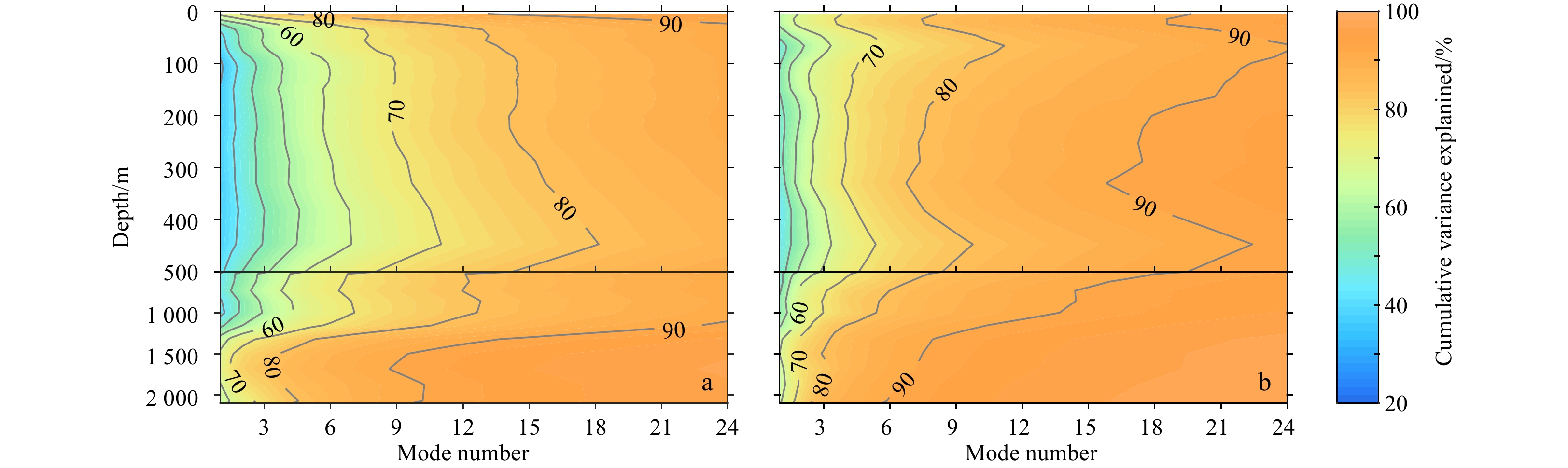
Figure 4. Cumulative contribution of different numbers of empirical orthogonal function leading modes to the total variance for temperature (a) and salinity (b) anomalies at different depths.
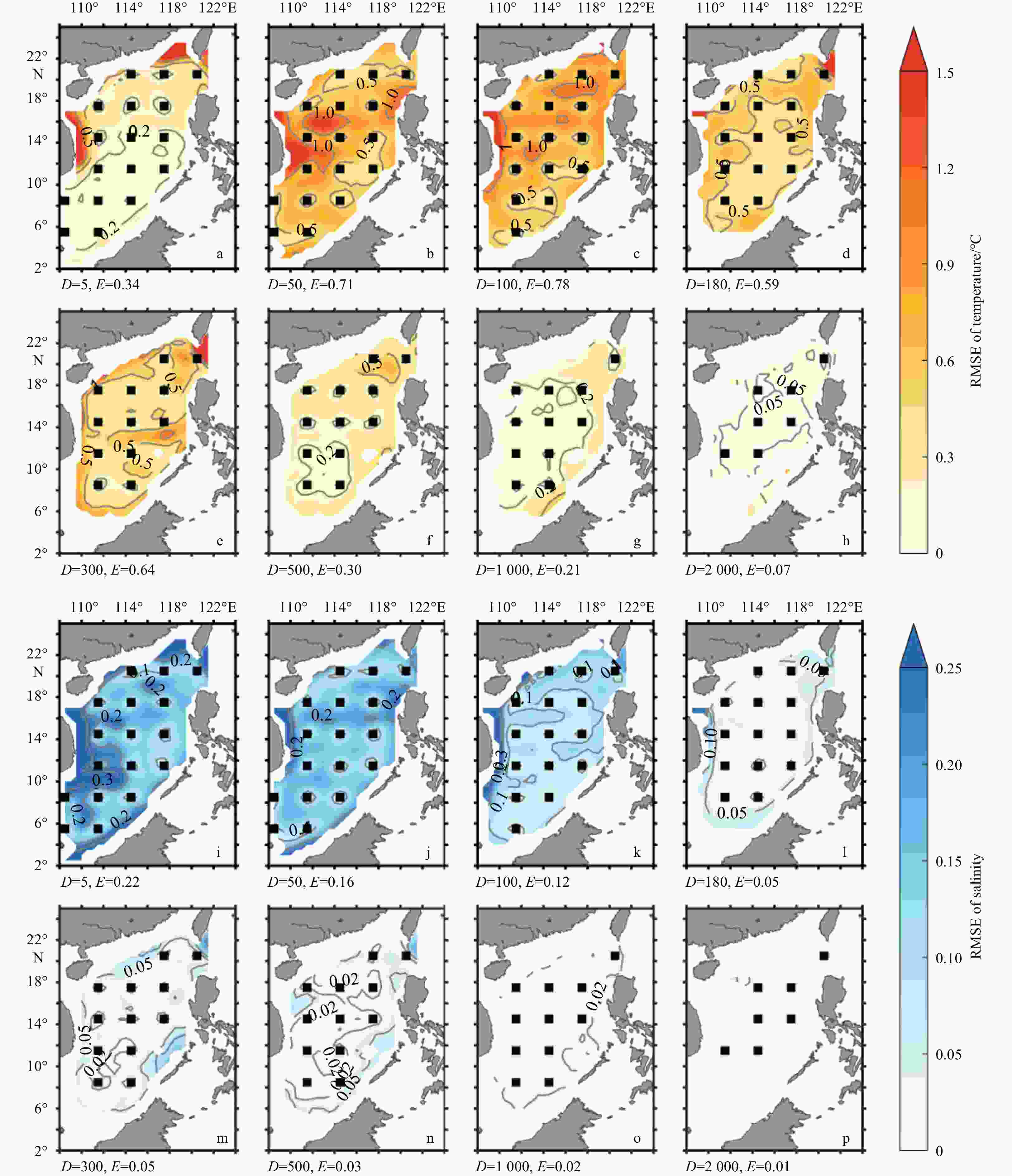
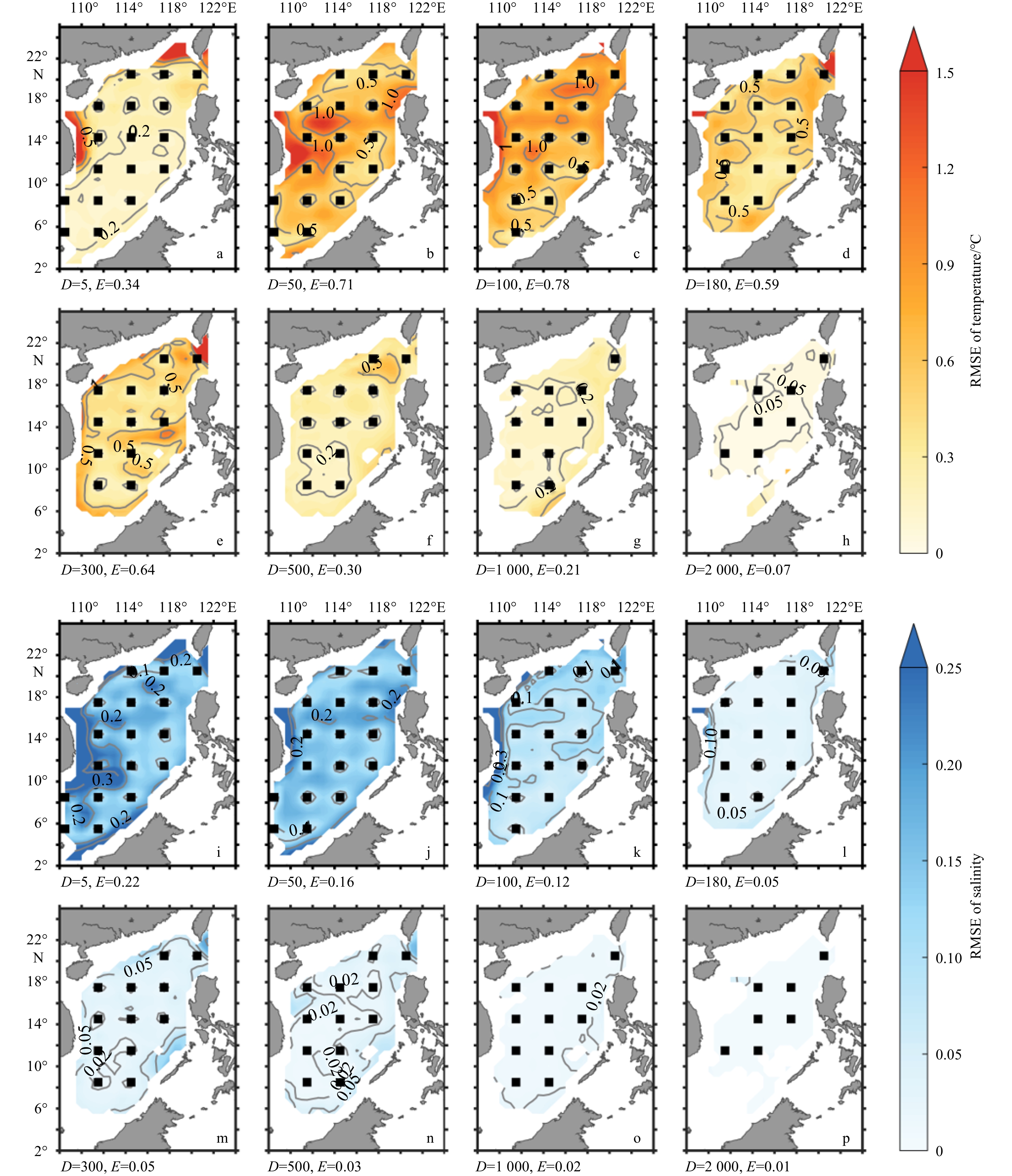
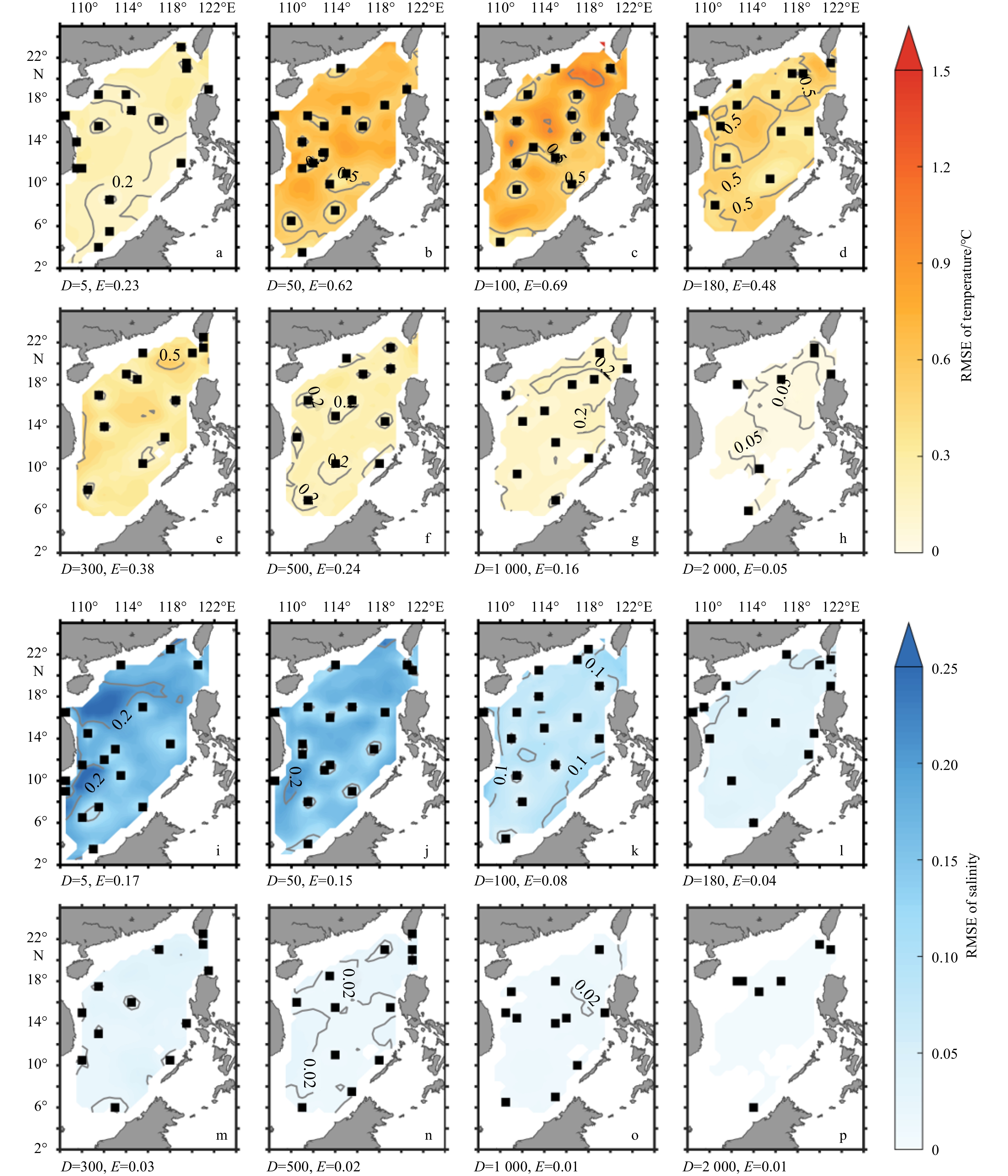
Figure 5. RMSEs of reconstructed temperature (a–h) and salinity (i–p) derived from the initial array at different depths. The black squares are the locations of the initial array. D and E in the sub-panels represent the depth (unit: m) and the corresponding area averaged RMSE, respectively.

Figure 6. RMSEs of reconstructed temperature (a–h) and salinity (i–p) derived from the optimal arrays at different depths. The black squares are the locations of the optimal arrays for each depth. D and E in the sub-panels represent the depth (unit: m) and the corresponding area averaged RMSE, respectively.
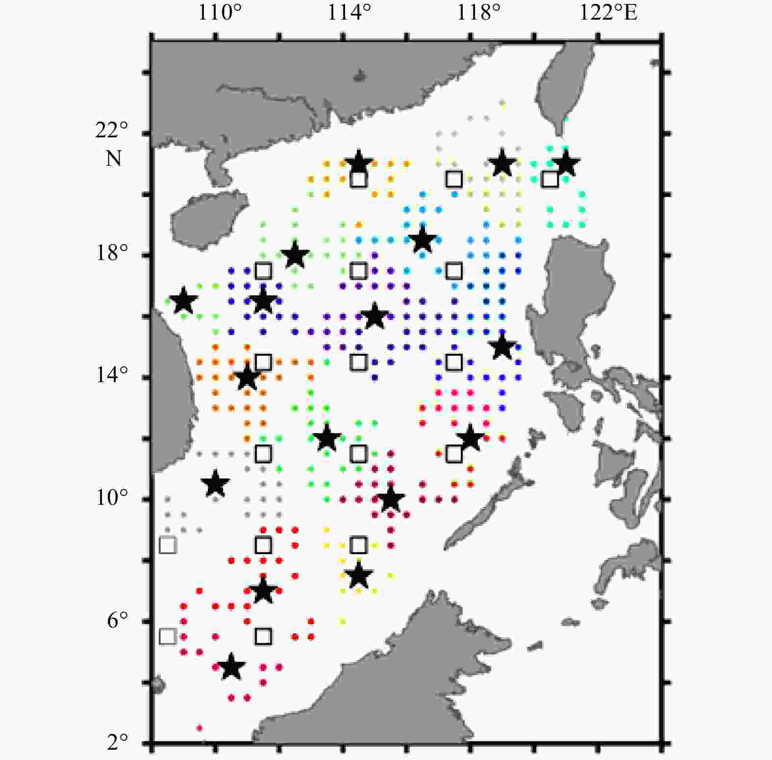
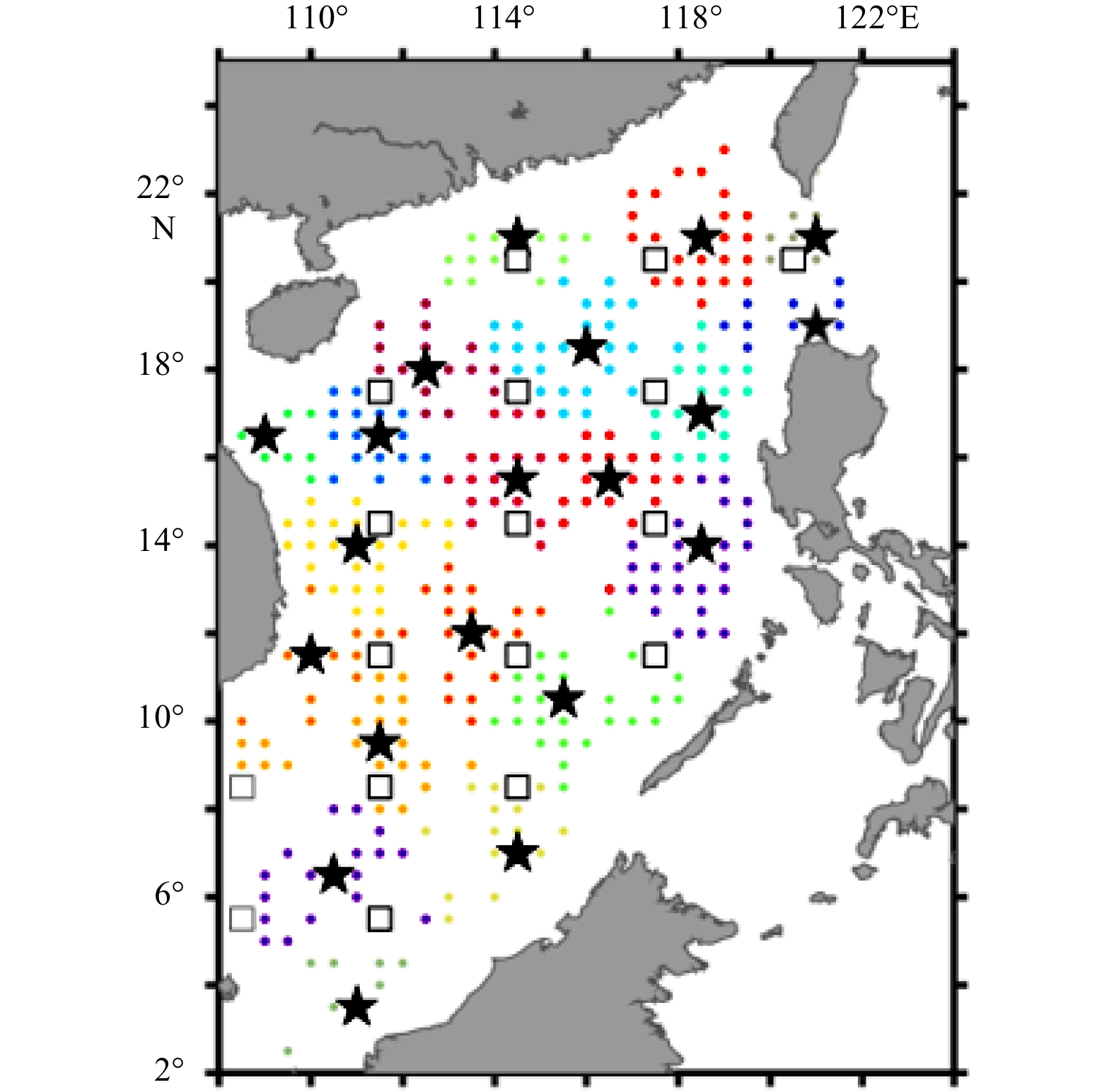
Figure 7. Consolidated array based on the K-center clustering algorithm. The solid stars indicate the clustered sites. The colored dots indicate locations for the optimal arrays at all depths, and different colors represent different categories in the K-center cluster.
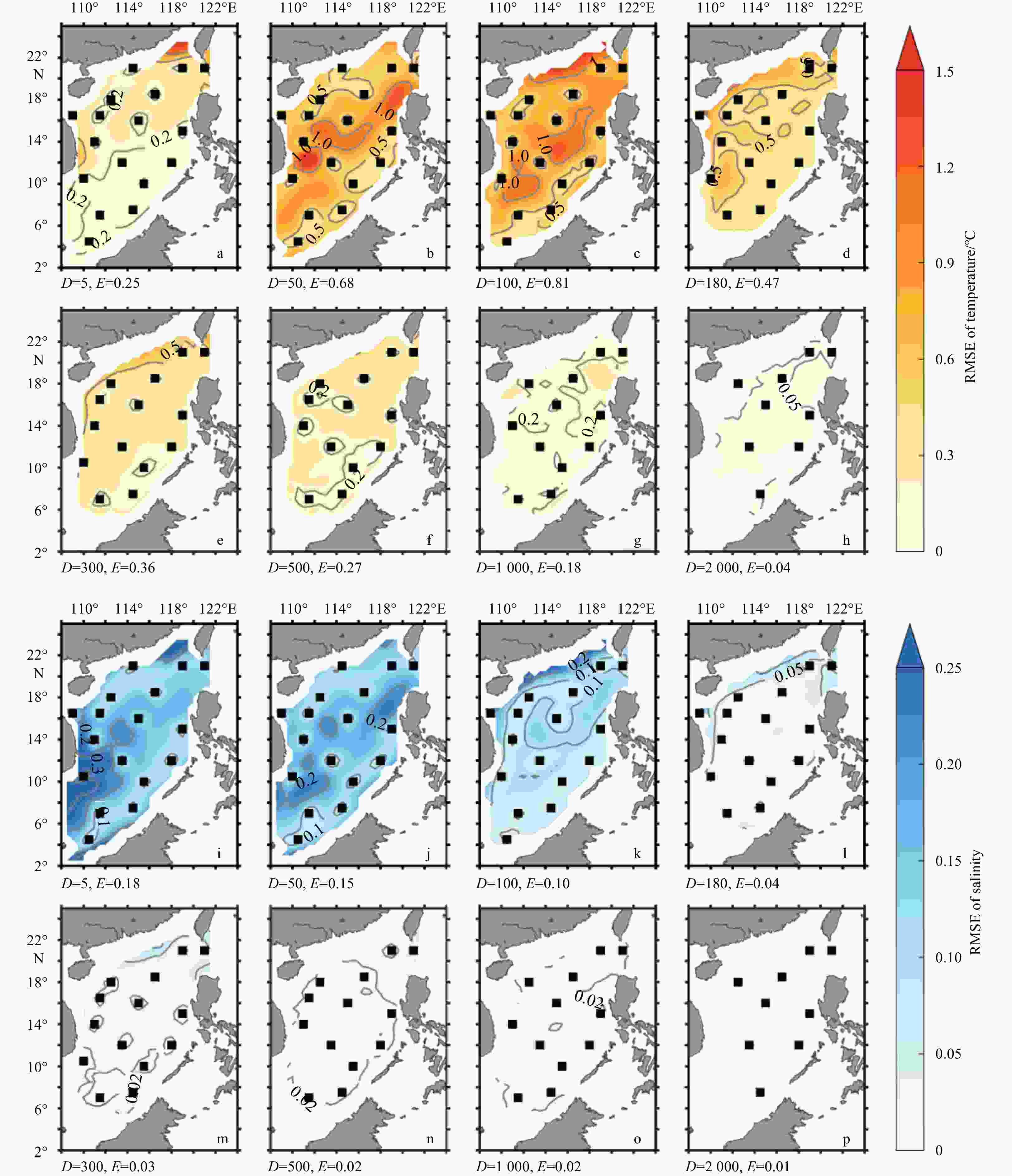
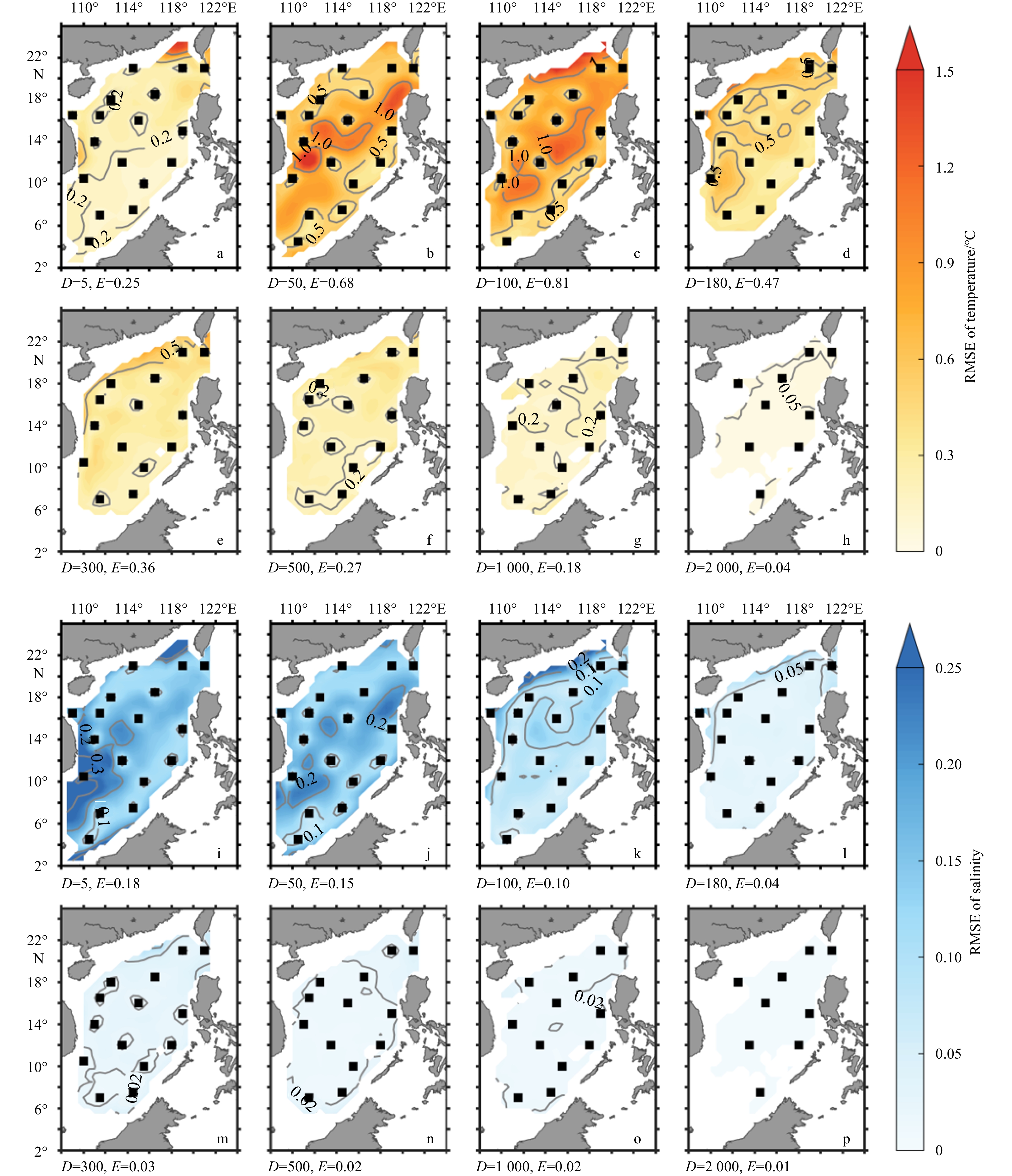
Figure 8. RMSEs of reconstructed temperature (a–h) and salinity (i–p) derived from the consolidated array at different depths. The black squares are the locations of the consolidated array. D and E in the sub-panels represent the depth (unit: m) and the corresponding area averaged RMSE, respectively.
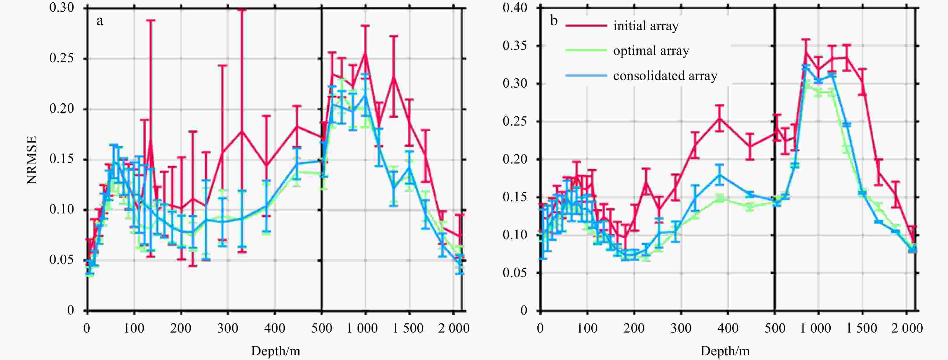
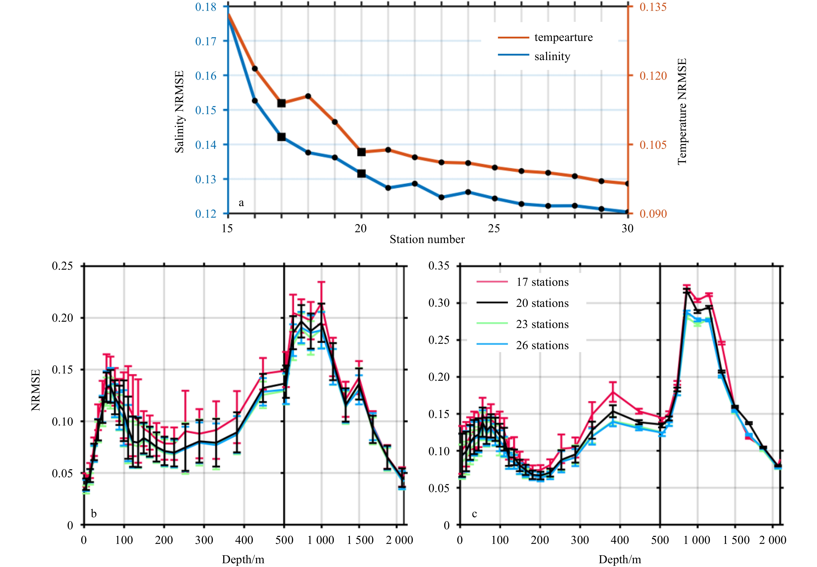
Figure 9. Area averaged RMSEs divided by corresponding ranges (normalized RMSEs, NRMSEs) at different depths in the South China Sea. a. Temperature; b. salinity. Vertical bars indicate the standard deviation of the NRMSEs.
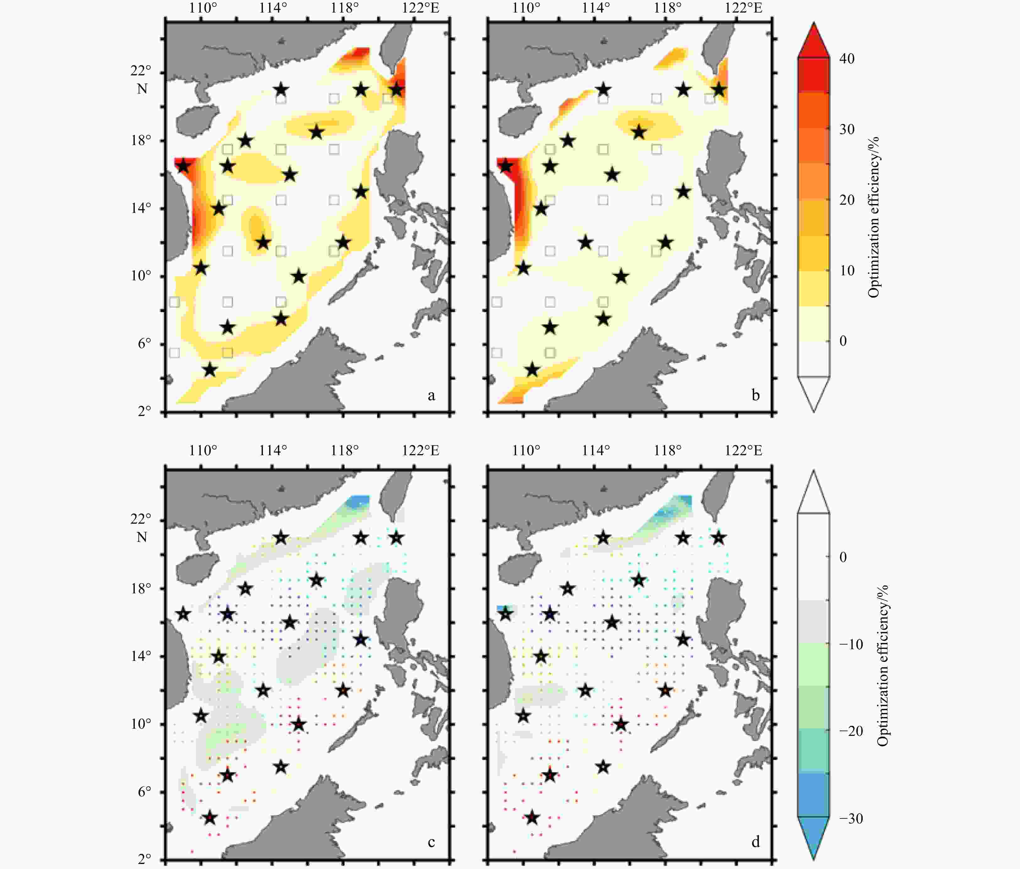
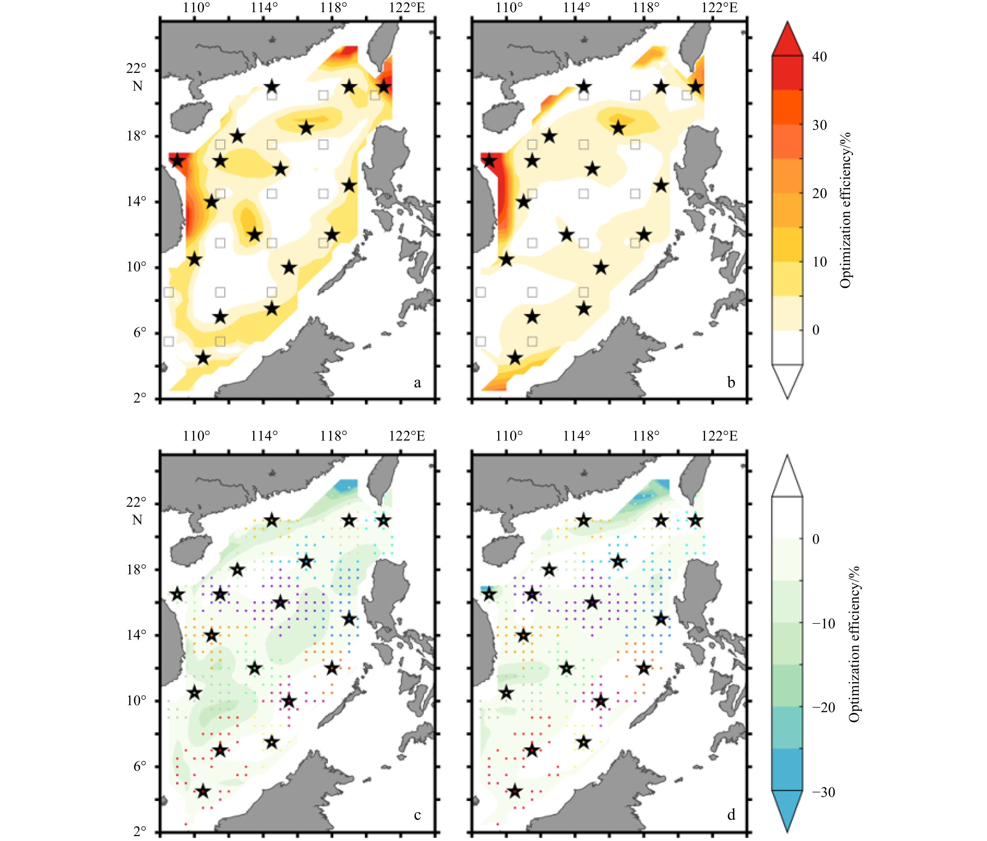
Figure 10. Optimization efficiency for temperature (a) and salinity (b) of the consolidated array in comparison with the initial array; c and d are the same as a and b but in comparison with the optimal arrays. The hollow squares and solid stars in a and b are the locations of initial and consolidated arrays, respectively. The colored dots in c and d indicate locations for the optimal arrays at all depths, and different colors represent different categories in the K-center cluster.

Figure 11. Averaged NRMSEs of temperature and salinity of the consolidated arrays with different site numbers (a), and NRMSEs of temperature (b) and salinity (c) at different depths in the South China Sea with consolidated arrays consist of 17, 20, 23, and 26 stations. Vertical bars in b and c indicate the standard deviation of the NRMSEs.
-
[1] Alvarez A, Mourre B. 2012. Optimum sampling designs for a glider-mooring observing network. Journal of Atmospheric and Oceanic Technology, 29(4): 601–612. doi: 10.1175/JTECH-D-11-00105.1 [2] Arnold C P Jr, Dey C H. 1986. Observing-systems simulation experiments: Past, present, and future. Bulletin of the American Meteorological Society, 67(6): 687–695. doi: 10.1175/1520-0477(1986)067<0687:OSSEPP>2.0.CO;2 [3] Ballabrera-Poy J, Hackert E, Murtugudde R, et al. 2007. An observing system simulation experiment for an optimal moored instrument array in the tropical Indian Ocean. Journal of Climate, 20(13): 3284–3299. doi: 10.1175/JCLI4149.1 [4] Carton J A, Chepurin G A, Chen Ligang. 2018. SODA3: a new ocean climate reanalysis. Journal of Climate, 31(17): 6967–6983. doi: 10.1175/JCLI-D-18-0149.1 [5] Fang Guohong, Chen Haiying, Wei Zexun, et al. 2006. Trends and interannual variability of the South China Sea surface winds, surface height, and surface temperature in the recent decade. Journal of Geophysical Research: Oceans, 111(C11): C11S16 [6] Feng Rong, Duan Wansuo, Mu Mu. 2017. Estimating observing locations for advancing beyond the winter predictability barrier of Indian Ocean dipole event predictions. Climate Dynamics, 48(3−4): 1173–1185. doi: 10.1007/s00382-016-3134-3 [7] Frolov S, Baptista A, Wilkin M. 2008. Optimizing fixed observational assets in a coastal observatory. Continental Shelf Research, 28(19): 2644–2658. doi: 10.1016/j.csr.2008.08.009 [8] Fu Weiwei, Høyer J L, She Jun. 2011. Assessment of the three dimensional temperature and salinity observational networks in the Baltic Sea and North Sea. Ocean Science, 7(1): 75–90. doi: 10.5194/os-7-75-2011 [9] Fujii Y, Rémy E, Zuo Hao, et al. 2019. Observing system evaluation based on ocean data assimilation and prediction systems: On-going challenges and a future vision for designing and supporting ocean observational networks. Frontiers in Marine Science, 6: 417. doi: 10.3389/fmars.2019.00417 [10] Gasparin F, Roemmich D, Gilson J, et al. 2015. Assessment of the upper-ocean observing system in the equatorial Pacific: The role of Argo in resolving intraseasonal to interannual variability. Journal of Atmospheric and Oceanic Technology, 32(9): 1668–1688. doi: 10.1175/JTECH-D-14-00218.1 [11] Geng Wu, Cheng Feng, Xie Qiang, et al. 2020. Observation system simulation experiments using an ensemble-based method in the northeastern South China Sea. Journal of Oceanology and Limnology, 38(6): 1729–1745. doi: 10.1007/s00343-019-9119-4 [12] Haber J, Zeilfelder F, Davydov O, et al. 2001. Smooth approximation and rendering of large scattered data sets. In: Proceedings of the Conference on Visualization. San Diego, CA: IEEE, 341–348 [13] Hackert E C, Miller R N, Busalacchi A J. 1998. An optimized design for a moored instrument array in the tropical Atlantic Ocean. Journal of Geophysical Research: Oceans, 103(C4): 7491–7509. doi: 10.1029/97JC03206 [14] Hirschi J, Baehr J, Marotzke J, et al. 2003. A monitoring design for the Atlantic meridional overturning circulation. Geophysical Research Letters, 30(7): 1413 [15] Hu Junya, Duan Wansuo. 2016. Relationship between optimal precursory disturbances and optimally growing initial errors associated with ENSO events: Implications to target observations for ENSO prediction. Journal of Geophysical Research: Oceans, 121(5): 2901–2917. doi: 10.1002/2015JC011386 [16] Hu Jianyu, Ho C R, Xie Lingling, et al. 2020. Regional Oceanography of the South China Sea. Singapore: World Scientific Publishing Company [17] Huang Xiaodong, Wang Zhaoyun, Zhang Zhiwei, et al. 2018. Role of mesoscale eddies in modulating the semidiurnal internal tide: Observation results in the northern South China Sea. Journal of Physical Oceanography, 48(8): 1749–1770. doi: 10.1175/JPO-D-17-0209.1 [18] Huang Xiaodong, Zhang Zhiwei, Zhang Xiaoqiang, et al. 2017. Impacts of a mesoscale eddy pair on internal solitary waves in the northern South China Sea revealed by mooring array observations. Journal of Physical Oceanography, 47(7): 1539–1554. doi: 10.1175/JPO-D-16-0111.1 [19] Lermusiaux P F J. 2007. Adaptive modeling, adaptive data assimilation and adaptive sampling. Physica D: Nonlinear Phenomena, 230(1−2): 172–196. doi: 10.1016/j.physd.2007.02.014 [20] Li Yineng, Peng Shiqiu, Liu Duanling. 2014. Adaptive observation in the South China Sea using CNOP approach based on a 3-D ocean circulation model and its adjoint model. Journal of Geophysical Research: Oceans, 119(12): 8973–8986. doi: 10.1002/2014JC010220 [21] Liang Zhanlin, Xing Tao, Wang Yinxia, et al. 2019. Mixed layer heat variations in the South China Sea observed by Argo float and reanalysis data during 2012–2015. Sustainability, 11(19): 5429. doi: 10.3390/su11195429 [22] Liu Danian, Zhu Jiang, Shu Yeqiang, et al. 2018a. Model-based assessment of a northwestern tropical Pacific moored array to monitor intraseasonal variability. Ocean Modelling, 126: 1–12. doi: 10.1016/j.ocemod.2018.04.001 [23] Liu Danian, Zhu Jiang, Shu Yeqiang, et al. 2018b. Targeted observation analysis of a northwestern tropical Pacific Ocean mooring array using an ensemble-based method. Ocean Dynamics, 68(9): 1109–1119. doi: 10.1007/s10236-018-1188-y [24] Masutani M, Schlatter T W, Errico R M, et al. 2010. Observing system simulation experiments. In: Lahoz W, Khattatov B, Menard R, eds. Data Assimilation: Making Sense of Observations. Berlin, Heidelberg: Springer, 647–679 [25] McIntosh P C. 1987. Systematic design of observational arrays. Journal of Physical Oceanography, 17(7): 885–902. doi: 10.1175/1520-0485(1987)017<0885:SDOOA>2.0.CO;2 [26] Mu Mu, Duan Wansuo. 2003. A new approach to studying ENSO predictability: Conditional nonlinear optimal perturbation. Chinese Science Bulletin, 48(10): 1045–1047. doi: 10.1007/BF03184224 [27] Oke P R, Sakov P. 2012. Assessing the footprint of a regional ocean observing system. Journal of Marine Systems, 105–108: 30–51 [28] Oke P R, Schiller A. 2007. A model-based assessment and design of a tropical Indian Ocean mooring array. Journal of Climate, 20(13): 3269–3283. doi: 10.1175/JCLI4170.1 [29] Palmer T N, Gelaro R, Barkmeijer J, et al. 1998. Singular vectors, metrics, and adaptive observations. Journal of the Atmospheric Sciences, 55(4): 633–653. doi: 10.1175/1520-0469(1998)055<0633:SVMAAO>2.0.CO;2 [30] Park H S, Jun C H. 2009. A simple and fast algorithm for K-medoids clustering. Expert Systems with Applications, 36(2): 3336–3341. doi: 10.1016/j.eswa.2008.01.039 [31] Peng Hanbang, Pan Aijun, Zheng Quanan et al. 2018. Analysis of monthly variability of thermocline in the South China Sea. Journal of Oceanology and Limnology, 36(2): 205–215. doi: 10.1007/s00343-017-6151-0 [32] Sakov P, Oke P R. 2008. Objective array design: Application to the tropical Indian Ocean. Journal of Atmospheric and Oceanic Technology, 25(5): 794–807. doi: 10.1175/2007JTECHO553.1 [33] Sun Zhongbin, Zhang Zhiwei, Qiu Bo, et al. 2020. Three-dimensional structure and interannual variability of the Kuroshio loop current in the northeastern South China Sea. Journal of Physical Oceanography, 50(9): 2437–2455. doi: 10.1175/JPO-D-20-0058.1 [34] Thomson R E, Emery W J. 2014. Data Analysis Methods in Physical Oceanography. 3rd ed. New York: Elsevier, 335–356 [35] Vecchi G A, Harrison M J. 2007. An observing system simulation experiment for the Indian Ocean. Journal of Climate, 20(13): 3300–3319. doi: 10.1175/JCLI4147.1 [36] Wang Zhaoyun, Huang Xiaodong, Yang Yunchao, et al. 2020. Impacts of subtidal motions and the earth rotation on modal characteristics of the semidiurnal internal tide. Journal of Oceanography, 76(1): 15–27. doi: 10.1007/s10872-019-00524-7 [37] Wei Zexun, Li Shujiang, Susanto R D, et al. 2019. An overview of 10-year observation of the South China Sea branch of the Pacific to Indian Ocean throughflow at the Karimata Strait. Acta Oceanologica Sinica, 38(4): 1–11. doi: 10.1007/s13131-019-1410-x [38] Xiao Fuan, Wang Dongxiao, Zeng Lili, et al. 2019. Contrasting changes in the sea surface temperature and upper ocean heat content in the South China Sea during recent decades. Climate Dynamics, 53(3−4): 1597–1612. doi: 10.1007/s00382-019-04697-1 [39] Xue Pengfei, Chen Changsheng, Beardsley R C, et al. 2011. Observing system simulation experiments with ensemble Kalman filters in Nantucket Sound, Massachusetts. Journal of Geophysical Research: Oceans, 116(C1): C01011 [40] Yang Qingxuan, Tian Jiwei, Zhao Wei. 2007. Observation of Luzon Strait transport in summer 2007. Deep-Sea Research Part I: Oceanographic Research Papers, 57(5): 670–676 [41] Yang Lei, Wang Dongxiao, Huang Jian, et al. 2015. Toward a mesoscale hydrological and marine meteorological observation network in the South China Sea. Bulletin of the American Meteorological Society, 96(7): 1117–1135. doi: 10.1175/BAMS-D-14-00159.1 [42] Yi Dalingli, Melnichenko O, Hacker P, et al. 2020. Remote sensing of sea surface salinity variability in the South China Sea. Journal of Geophysical Research: Oceans, 125(12): e2020JC016827 [43] Yildirim B, Chryssostomidis C, Karniadakis G E. 2009. Efficient sensor placement for ocean measurements using low-dimensional concepts. Ocean Modelling, 27(3–4): 160–173. doi: 10.1016/j.ocemod.2009.01.001 [44] Zeng Lili, Wang Qiang, Xie Qiang, et al. 2015. Hydrographic field investigations in the northern South China Sea by open cruises during 2004–2013. Science Bulletin, 60(6): 607–615. doi: 10.1007/s11434-015-0733-z [45] Zhang Yanwu, Bellingham J G. 2008. An efficient method of selecting ocean observing locations for capturing the leading modes and reconstructing the full field. Journal of Geophysical Research: Oceans, 113(C4): C04005 [46] Zhang Kun, Mu Mu, Wang Qiang. 2017. Identifying the sensitive area in adaptive observation for predicting the upstream Kuroshio transport variation in a 3-D ocean model. Science China Earth Sciences, 60(5): 866–875. doi: 10.1007/s11430-016-9020-8 [47] Zhang Kun, Mu Mu, Wang Qiang, et al. 2019. CNOP-based adaptive observation network designed for improving upstream Kuroshio transport prediction. Journal of Geophysical Research: Oceans, 124(6): 4350–4364. doi: 10.1029/2018JC014490 [48] Zhang Kun, Mu Mu, Wang Qiang. 2020. Increasingly important role of numerical modeling in oceanic observation design strategy: A review. Science China Earth Sciences, 63(11): 1678–1690. doi: 10.1007/s11430-020-9674-6 [49] Zhang Zhiwei, Zhao Wei, Tian Jiwei, et al. 2015. Spatial structure and temporal variability of the zonal flow in the Luzon Strait. Journal of Geophysical Research: Oceans, 120(2): 759–776. doi: 10.1002/2014JC010308 [50] Zhao Wei, Zhou Chun, Tian Jiwei, et al. 2014. Deep water circulation in the Luzon Strait. Journal of Geophysical Research: Oceans, 119(2): 790–804. doi: 10.1002/2013JC009587 [51] Zhou Chun, Zhao Wei, Tian Jiwei, et al. 2017. Deep western boundary current in the South China Sea. Scientific Reports, 7: 9303. doi: 10.1038/s41598-017-09436-2 [52] Zhu Yaohua, Fang Guohong, Wei Zexun, et al. 2016. Seasonal variability of the meridional overturning circulation in the South China Sea and its connection with inter-ocean transport based on SODA2.2.4. Journal of Geophysical Research: Oceans, 121(5): 3090–3105. doi: 10.1002/2015JC011443 -

 下载:
下载:

 点击查看大图
计量
- 文章访问数: 339
- HTML全文浏览量: 93
- PDF下载量: 16
- 被引次数: 0