

Vertical multiple-layer structure of temperature and turbulent diffusivity in the South China Sea
-
Abstract: We report field measurements of vertical profiles of the turbulent diffusivity and temperature at different stations in the South China Sea (SCS). Our study shows that the measured turbulent diffusivity follows a power-law distribution with a varying exponent in water layers. Similar multiple-layer scaling regimes were also observed from the temperature fluctuations. Combining turbulent diffusivity and temperature fluctuations, the vertical structure of temperature was revealed. Furthermore, we discussed the temperature profiles in each layer. A constant function of a dimensionless temperature profile was found in water layers that have identical turbulence conditions. Our results reveal the multiple-layer structure of temperature in the SCS. This study contributes to the understanding of the vertical structure of multiple layers in the SCS and provides clues for exploring the physical mechanism for maintaining the temperature structure.
-
Key words:
- temperature profile /
- turbulent diffusivity /
- South China Sea /
- multiple layers
-

Figure 1. Sketch of the measurement locations of local temperature and velocity shear in the SCS: Stas s1–s8 denote the locations of temperature data from CTD measurements along the section of 18°N; Stas q1–q5 are for the CTD data in the SCS central basin; Sta. kj1 is for the CTD data at the slope of the northern SCS; Stas c1–c9 are for the velocity shear data from VMP-X measurements with
$ z $ up to 3900 m. Asterisks denote velocity shear data from TurboMAP measurements where$ z < 500\;\mathrm{m} $ . Gray lines denote isobaths in meters.
Figure 2. Overview of vertical profiles of temperature in the section of 18°N (a), the central basin of the SCS (b), and the slope of the northern SCS (c).

Figure 3. Measured
$ {\kappa }_{\rho } \left(z\right) $ from 44 stations in the upper ocean (a) and direct kernel smoothing probability density distribution of the measured$ {\kappa }_{\rho } \left(z\right) $ in a for different values of$ z $ (b). The solid curve in a is the algebraic average value of$ {\kappa }_{\rho } $ .
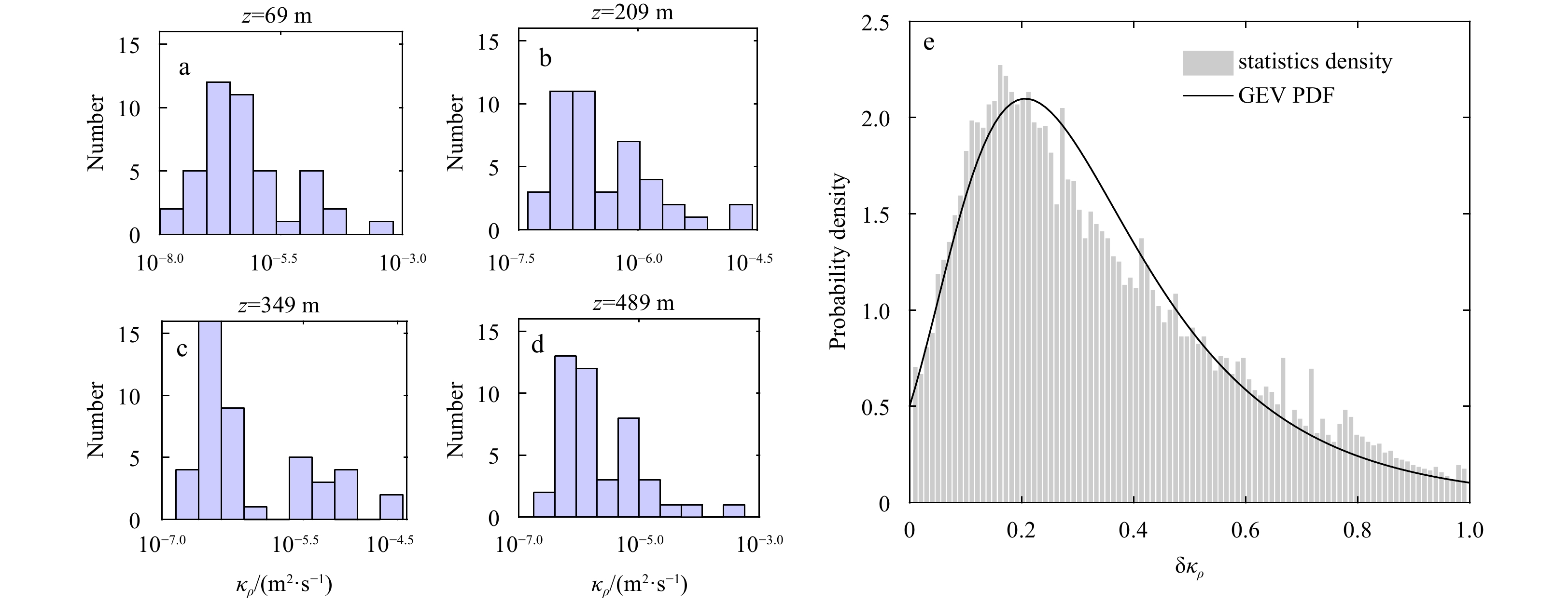
Figure 4. Statistics of diffusivity in 10 segmentations of measured ranges at 69 m (a), 209 m (b), 349 m (c) and 489 m (d), and statistics density of diffusivity in 100 segmentations of measured ranges at all depths (e). The black solid curve in e shows the generalized extreme value (GEV) probability density function (PDF).

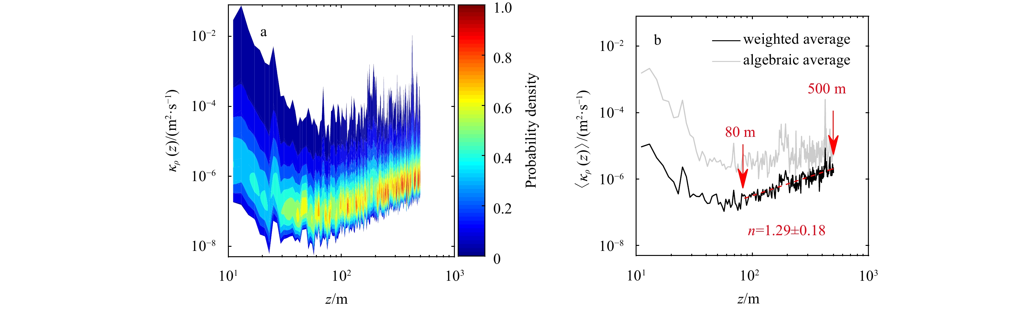
Figure 5. Generalized extreme value probability density distribution with
$ z $ (a) and the algebraic average values and weighted average value$ \left\langle{{\kappa }_{\rho }\left(z\right)}\right\rangle $ with$ z $ (b). The red dotted curve is the fitting curve of the weighted average value for 80 m<z<500 m.
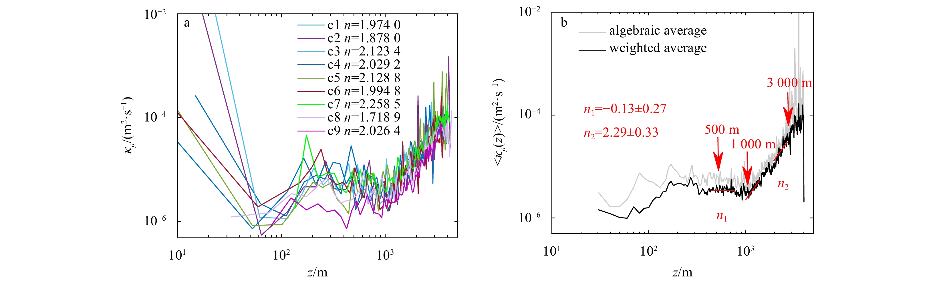
Figure 6. The profiles of
$ {\kappa }_{\rho } $ and the$ n $ values of the power-law fit for 1 000 m<z<3 000 m from Stas c1–c9 (a) and the weighted average and algebraic average values of$ {\kappa }_{\rho } $ in a (b). The red dotted curves are the power-law fitting curves. n1 and n2 are the$ n $ values of the power-law$ \left\langle{{\kappa }_{\rho }\left(z\right)}\right\rangle\sim {z}^{n} $ from the weighted average$ {\kappa }_{\rho } $ profile for$ 500\;\mathrm{m} < z < 1\;000\;\mathrm{m} $ and$ 1\;000\;\mathrm{m} < z < 3\;000\;\mathrm{m} $ , respectively.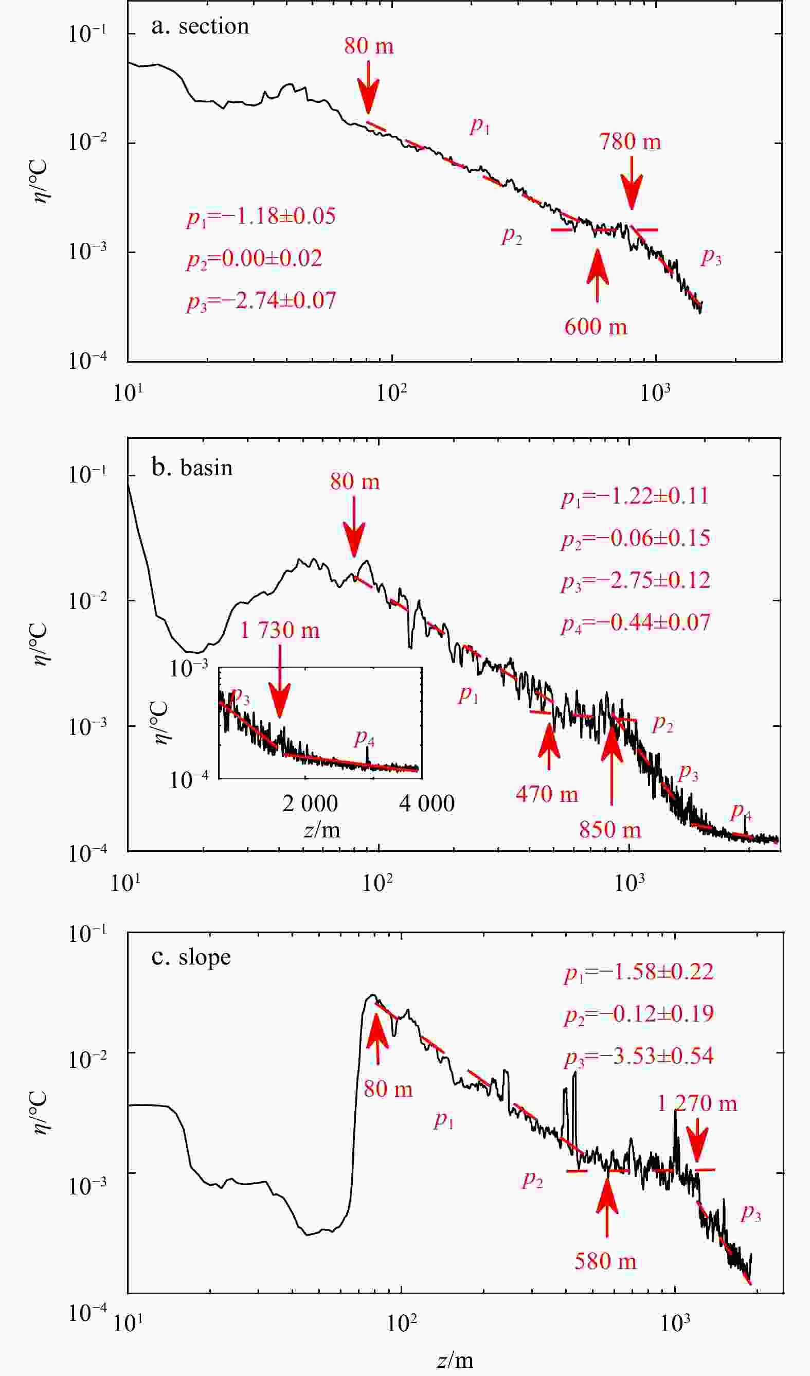
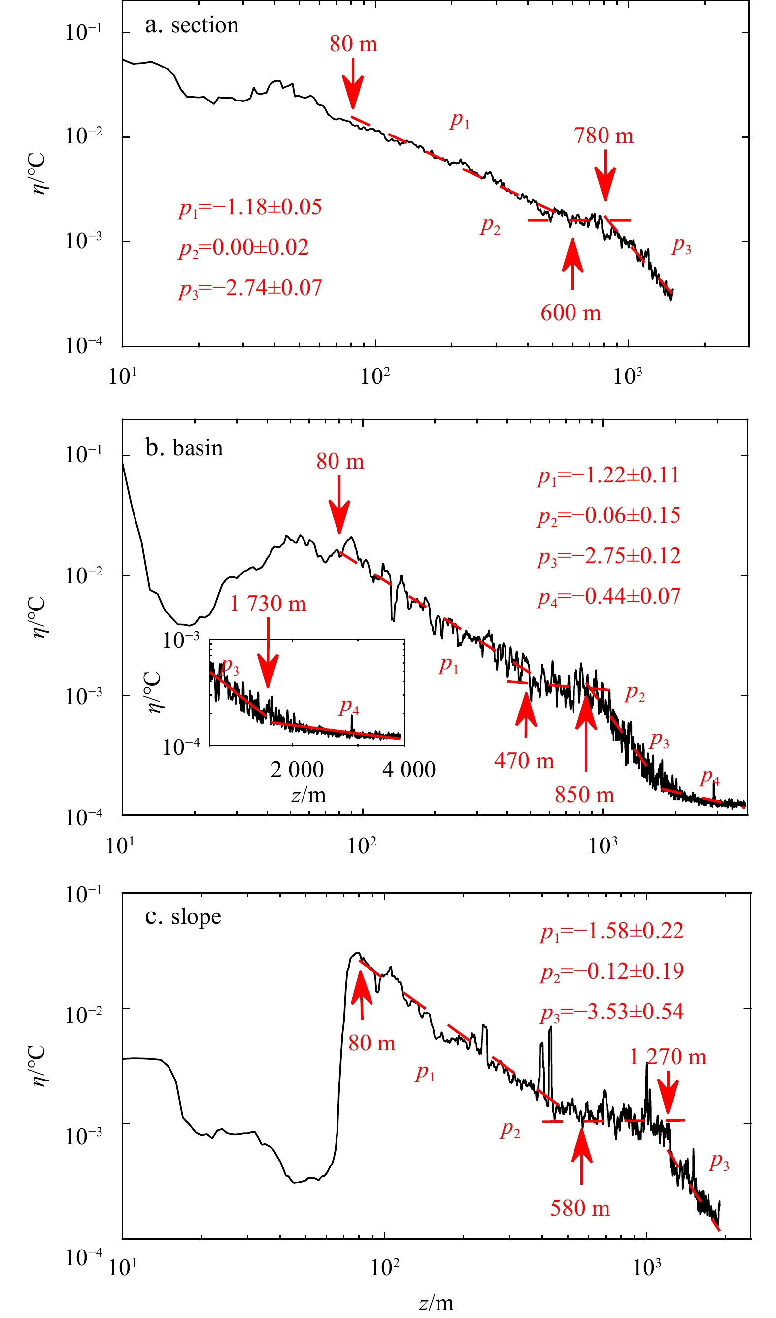
Figure 7. Measured temperature root-mean-square profile
$\eta \left(z\right)$ in the section of 18°N (a), the central basin of the SCS (b) and the slope of the northern SCS (c). The red dotted curves are the power-law fitting curves. The inset in b shows an expanded view of the profile for$z > 1\;200$ m. p1, p2, p3 and p4 are the$ p $ values of the power-law$\eta \left(z\right) \sim {z}^{p}$ in the upper layer, transition layer, middle layer, and deep layer, respectively.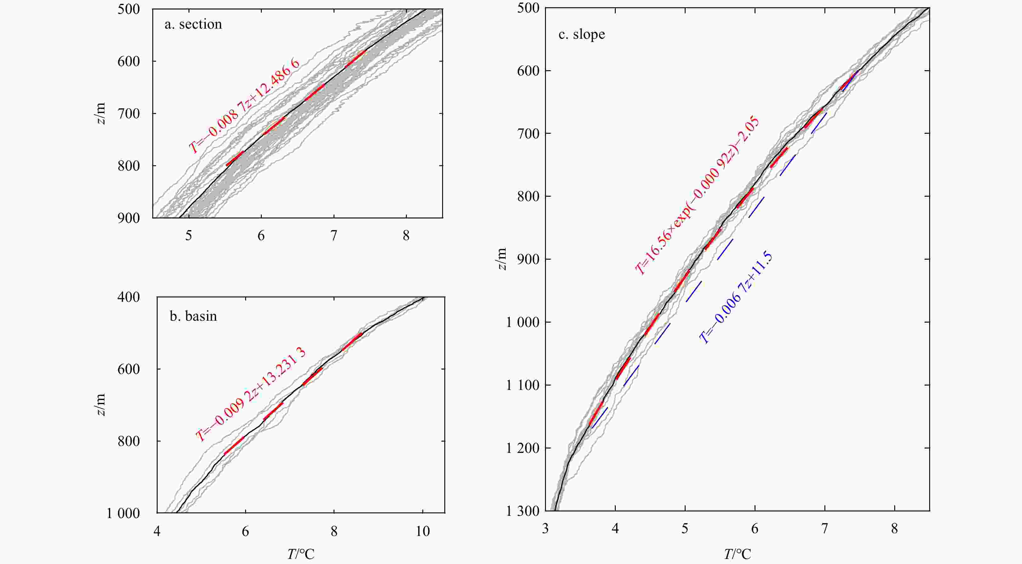
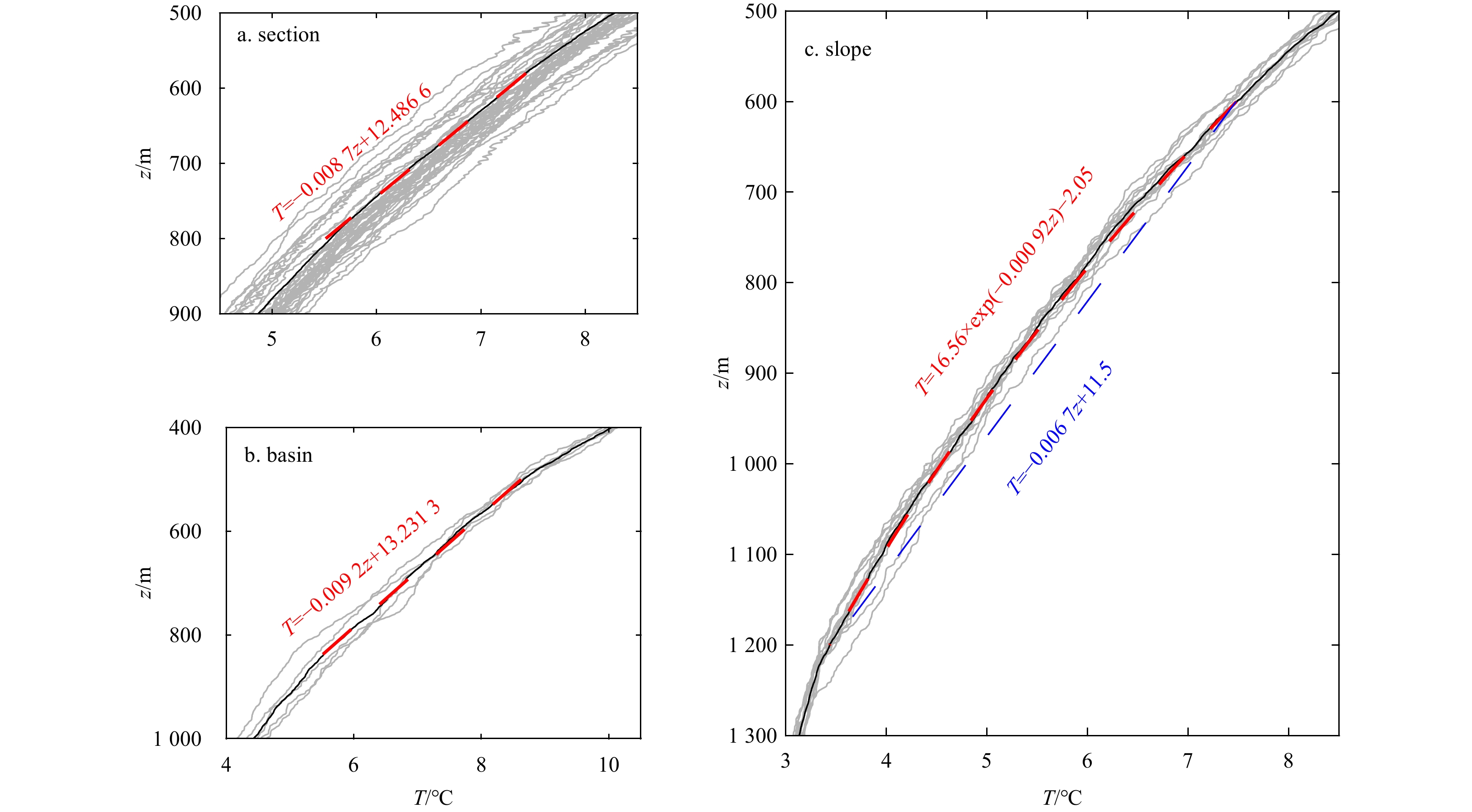
Figure 8. Measured temperature profiles (grey curves), averaged temperature profile (black curve), and fitting temperature profile of the transition layer (red dotted line) in the section of 18°N (a), the central basin in the SCS (b), and the slope of the northern SCS (c), respectively. The blue dotted line is the linear fitting temperature profile of the transition layer in slope.
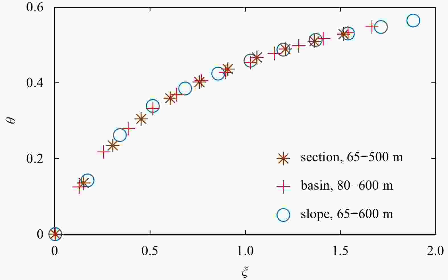
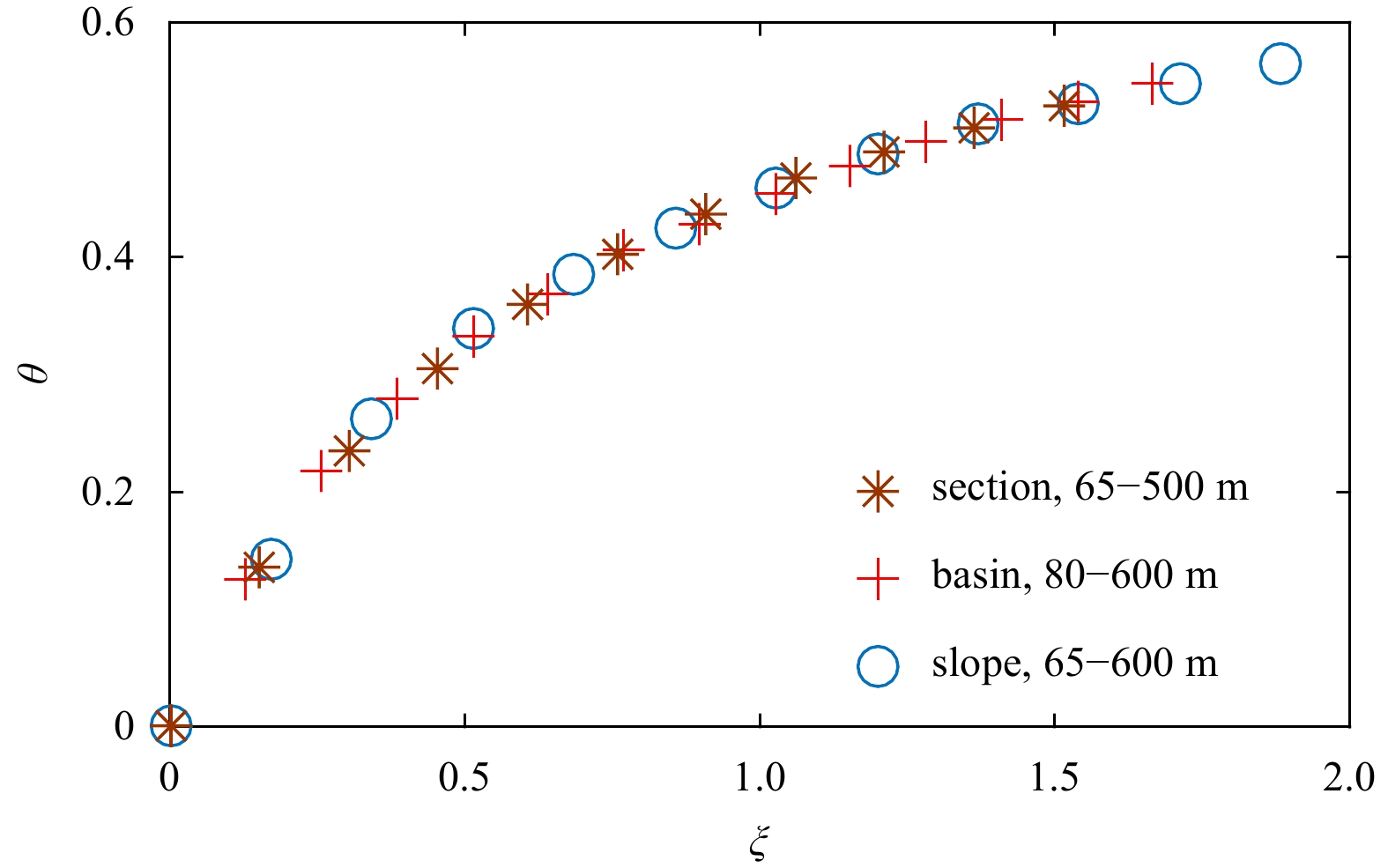
Figure 9. Dimensionless temperature profiles of upper layer in the section of 18°N, the central basin in the SCS, and the slope of the northern SCS.
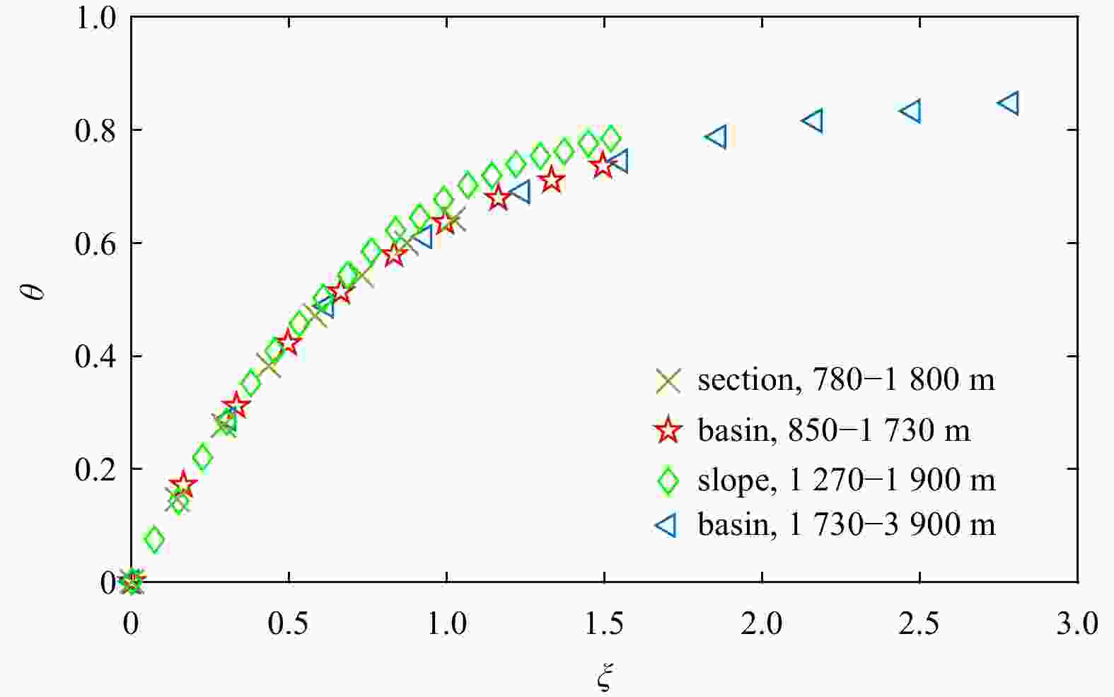
Figure 10. Dimensionless temperature profiles of middle layer in the section, basin, slope, and deep layer in the basin.
Table 1. Depth ranges of water layers
Area or source ZS of water layer/m UL TL ML DL Section of 18°N 80−600 600−780 780 to NAN NAN Central basin
in the SCS65−470 470−850 850−1730 1730 to NAN Slope of the
northern SCS80−580 580−1270 1270 to NAN NAN $ \left\langle{{\mathit{\kappa }}_{\mathit{\rho }}\left(\mathit{z}\right)}\right\rangle $ 80−500 500−1000 1000 to NAN NAN Model
(Gan et al., 2016)0−750 NAN 750−1500 1500 to NAN Note: NAN means no data. UL: upper layer, TL: transition layer, ML: middle layer, and DL: deep layer.  下载: 导出CSV
Table 2. Adjusted parameters for each layer
Region Water layer Parameter $ \Delta \mathit{T} $/°C $ {\mathit{L}}_{\mathit{\lambda }} $/m Section of 18°N UL 26.9 330 ML 4.4 618 Central basin in the SCS UL 27.8 234 ML 3.8 541 Slope of the northern SCS DL 0.5 645 UL 29.8 175 ML 0.9 394
下载: 导出CSV
-
Chu P C, Edmons N L, Fan Chenwu. 1999. Dynamical mechanisms for the South China Sea seasonal circulation and thermohaline variabilities. Journal of Physical Oceanography, 29(11): 2971–2989. doi: 10.1175/1520-0485(1999)029<2971:DMFTSC>2.0.CO;2 Gan Jianping, Liu Zhiqiang, Hui C R. 2016. A three-layer alternating spinning circulation in the South China Sea. Journal of Physical Oceanography, 46(8): 2309–2315. doi: 10.1175/JPO-D-16-0044.1 Golosov S, Zverev I, Shipunova E, et al. 2018. Modified parameterization of the vertical water temperature profile in the FLake model. Tellus A: Dynamic Meteorology and Oceanography, 70(1): 1–7 Hu Jianyu, Kawamura H, Hong Huasheng, et al. 2000. A review on the currents in the South China Sea: Seasonal circulation, South China Sea Warm Current and Kuroshio Intrusion. Journal of Oceanography, 56(6): 607–624. doi: 10.1023/A:1011117531252 Kitaigorodskii S A, Miropolskii Y Z. 1970. On the theory of active layer of open ocean. Atmospheric and Oceanic Physics, 6(2): 97–102 Lan Jian, Zhang Ningning, Wang Yu. 2013. On the dynamics of the South China Sea deep circulation. Journal of Geophysical Research, 118(3): 1206–1210. doi: 10.1002/jgrc.20104 Li Li, Qu Tangdong. 2006. Thermohaline circulation in the deep South China Sea basin inferred from oxygen distributions. Journal of Geophysical Research, 111(C5): C05017. doi: 10.1029/2005JC003164 Liang Changrong, Chen Guiying, Shang Xiaodong. 2017. Observations of the turbulent kinetic energy dissipation rate in the upper central South China Sea. Ocean Dynamics, 67(5): 597–609. doi: 10.1007/s10236-017-1051-6 Liu Qinyu, Yang Haijun, Liu Zhengyu. 2001. Seasonal features of the Sverdrup circulation in the South China Sea. Progress in Natural Science, 11(3): 202–206 Munk W H. 1966. Abyssal recipes. Deep-Sea Research and Oceanographic Abstracts, 13(4): 707–730. doi: 10.1016/0011-7471(66)90602-4 Osborn T R. 1980. Estimates of the local rate of vertical diffusion from dissipation measurements. Journal of Physical Oceanography, 10(1): 83–89. doi: 10.1175/1520-0485(1980)010<0083:EOTLRO>2.0.CO;2 Qu Tangdong, Girton J B, Whitehead J A. 2006. Deepwater overflow through Luzon Strait. Journal of Geophysical Research, 111(C1): C01002. doi: 10.1029/2005JC003139 Shang Xiaodong, Liang Changrong, Chen Guiying. 2017a. Spatial distribution of turbulent mixing in the upper ocean of the South China Sea. Ocean Science, 13(3): 503–519. doi: 10.5194/os-13-503-2017 Shang Xiaodong, Qi Yongfeng, Chen Guiying, et al. 2017b. An expendable microstructure profiler for deep ocean measurements. Journal of Atmospheric and Oceanic Technology, 34(1): 153–165. doi: 10.1175/JTECH-D-16-0083.1 Shaw P T, Chao S Y, Fu L L. 1999. Sea surface height variations in the South China Sea from satellite altimetry. Oceanologica Acta, 22(1): 1–17. doi: 10.1016/S0399-1784(99)80028-0 Shu Yeqiang, Xue Huijie, Wang Dongxiao, et al. 2014. Meridional overturning circulation in the South China Sea envisioned from the high-resolution global reanalysis data GLBa0.08. Journal of Geophysical Research, 119(5): 3012–3028. doi: 10.1002/2013JC009583 Su Jilan. 2004. Overview of the South China Sea circulation and its influence on the coastal physical oceanography outside the Pearl River Estuary. Continental Shelf Research, 24(16): 1745–1760. doi: 10.1016/j.csr.2004.06.005 Thorpe S A. 2005. The measurement of turbulence and mixing. In: Thorpe S A, ed. The Turbulent Ocean. Cambridge, UK: Cambridge University Press, 172–189 Tian Jiwei, Yang Qingxuan, Liang Xinfeng, et al. 2006. Observation of Luzon Strait transport. Geophysical Research Letters, 33(19): L19607. doi: 10.1029/2006GL026272 Tian Jiwei, Yang Qingxuan, Zhao Wei. 2009. Enhanced diapycnal mixing in the South China Sea. Journal of Physical Oceanography, 39(12): 3191–3203. doi: 10.1175/2009JPO3899.1 Wang Guihua, Xie Shangping, Qu Tangdong, et al. 2011. Deep South China Sea circulation. Geophysical Research Letters, 38(5): L05601. doi: 10.1029/2010GL046626 Wolk F, Yamazaki H, Seuront L, et al. 2002. A new free-fall profiler for measuring biophysical microstructure. Journal of Atmospheric and Oceanic Technology, 19(5): 780–793. doi: 10.1175/1520-0426(2002)019<0780:ANFFPF>2.0.CO;2 Wyrtki Klaus. 1961. Physical oceanography of the Southeast Asian waters: scientific results of marine investigations of the South China Sea and the Gulf of Thailand 1959–1961. NAGA Report, 2: 195. doi: 10.1530/jrf.0.0020195 Xie Qiang, Xiao Jingen, Wang Dongxiao, et al. 2013. Analysis of deep-layer and bottom circulations in the South China Sea based on eight quasi-global ocean model outputs. Chinese Science Bulletin, 58(32): 4000–4011. doi: 10.1007/s11434-013-5791-5 Yuan Dongliang. 2002. A numerical study of the South China Sea deep circulation and its relation to the Luzon Strait transport. Acta Oceanologica Sinica, 21(2): 187–202 -


 点击查看大图

计量
- 文章访问数: 735
- HTML全文浏览量: 256
- PDF下载量: 37
- 被引次数: 0