

-
Abstract: The near-inertial waves (NIWs) are important for energy cascade in the ocean. They are usually significantly reinforced by strong winds, such as typhoon. Due to relatively coarse resolutions in contemporary climate models, NIWs and associated ocean mixing need to be parameterized. In this study, a parameterization for NIWs proposed by Jochum in 2013 (J13 scheme), which has been widely used, is compared with the observations in the South China Sea, and the observations are treated as model outputs. Under normal conditions, the J13 scheme performs well. However, there are noticeable discrepancies between the J13 scheme and observations during typhoon. During Typhoon Kalmaegi in 2014, the inferred value of the boundary layer is deeper in the J13 scheme due to the weak near-inertial velocity shear in the vertical. After typhoon, the spreading of NIWs beneath the upper boundary layer is much faster than the theoretical prediction of inertial gravity waves, and this fast process is not rendered well by the J13 scheme. In addition, below the boundary layer, NIWs and associated diapycnal mixing last longer than the direct impacts of typhoon on the sea surface. Since the energy dissipation and diapycnal mixing below the boundary layer are bounded to the surface winds in the J13 scheme, the prolonged influences of typhoon via NIWs in the ocean interior are missing in this scheme. Based on current examination, modifications to the J13 scheme are proposed, and the modified version can reduce the discrepancies in the temporal and vertical structures of diapycnal mixing.
-
Key words:
- near-inertial waves /
- parameterization /
- ocean mixing /
- upper ocean boundary layer /
- typhoon
-
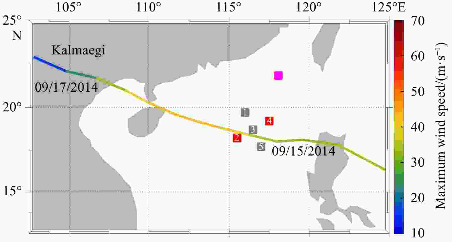
Figure 1. Five buoys deployed in the South China Sea in 2014 and the trajectory of typhoon Kalmaegi. The locations of the buoys are listed in Table 1. Buoys #2 and #4 are used in this study and they are marked with red squares. Other three buoys (gray squares) were destroyed by the typhoon and the data were not complete. The purple square denotes the location of observations using the VMP-250 in 2019. The colors on the typhoon trajectory indicate the maximum wind speed.
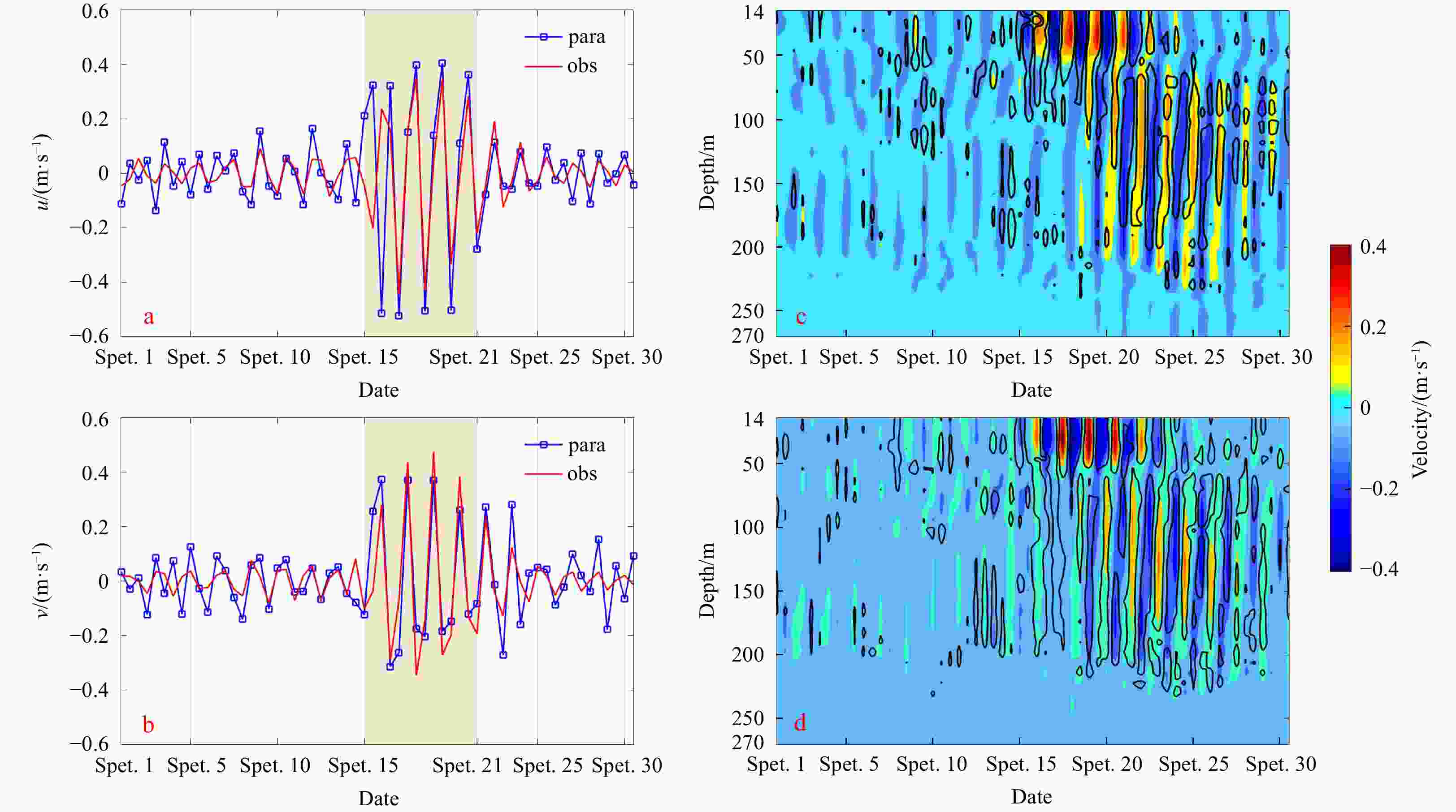
Figure 2. The comparison of near-inertial velocities. In a, the red line shows
$ {u}_{{\rm{obs}}}^{i} $ at 22 m and Buoy #2, which is obtained with a Butterworth bandpass filter between 0.7f and 1.3f; the blue line shows the corresponding$ {u}_{{\rm{para}}}^{i} $ obtained with Eq. (4a) after a 12-h running mean. In b, the red line and blue line are for$ {v}_{{\rm{obs}}}^{i} $ and$ {v}_{{\rm{para}}}^{i} $ at 22 m and Buoy #2. c shows the comparisons between$ {u}_{{\rm{obs}}}^{i} $ (colors) and$ {u}_{{\rm{para}}}^{i} $ (black contours) at Buoy #2. d is the same as c but for the comparisons between$ {v}_{{\rm{obs}}}^{i} $ (colors) and$ {v}_{{\rm{para}}}^{i} $ (black contours). The yellow shades in a and b are from September 15 to 21, when the wind speed is larger than 30 m/s and typhoon Kalmaegi had a direct impact on the buoy array. Para: parameterization, obs: observation.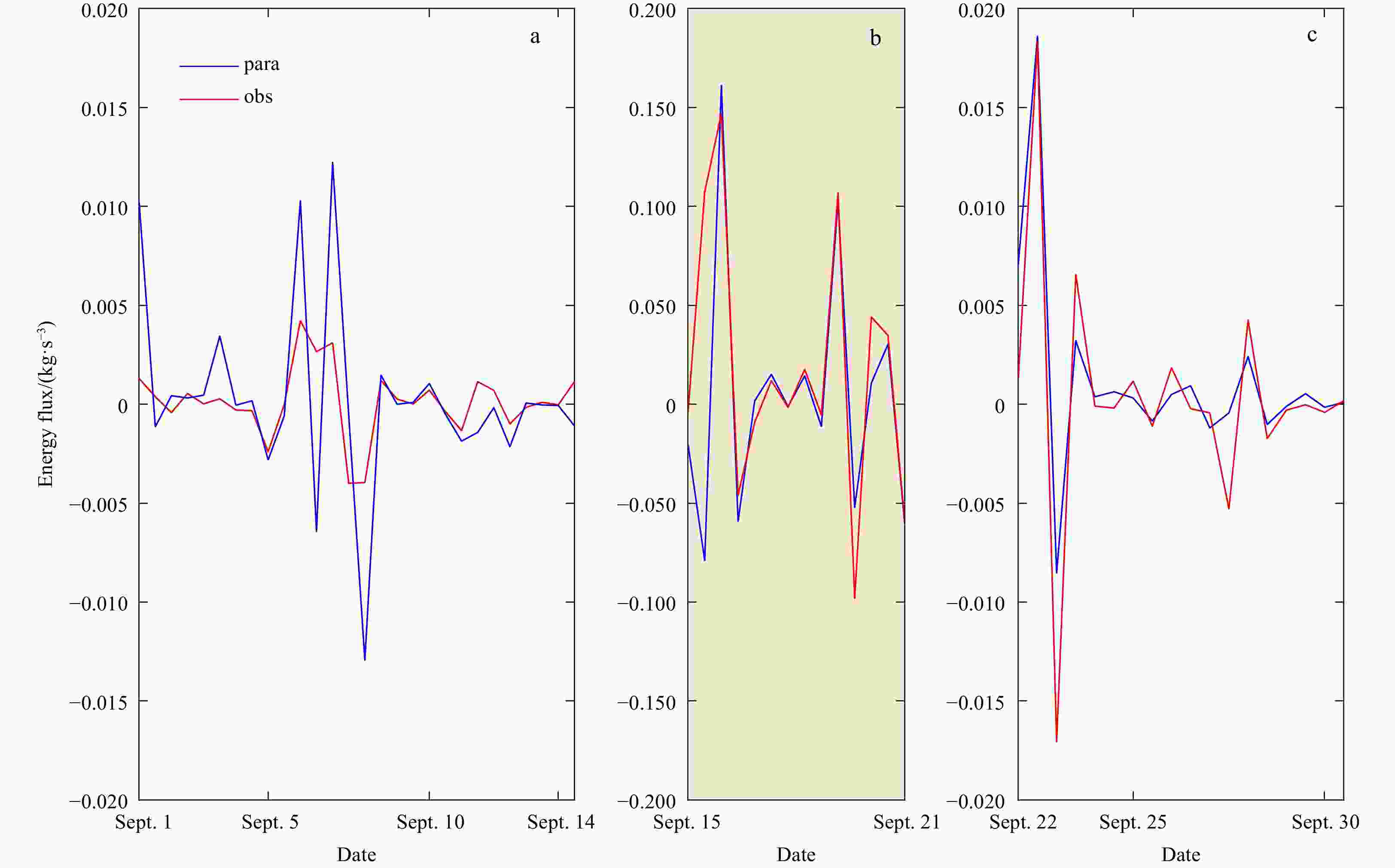
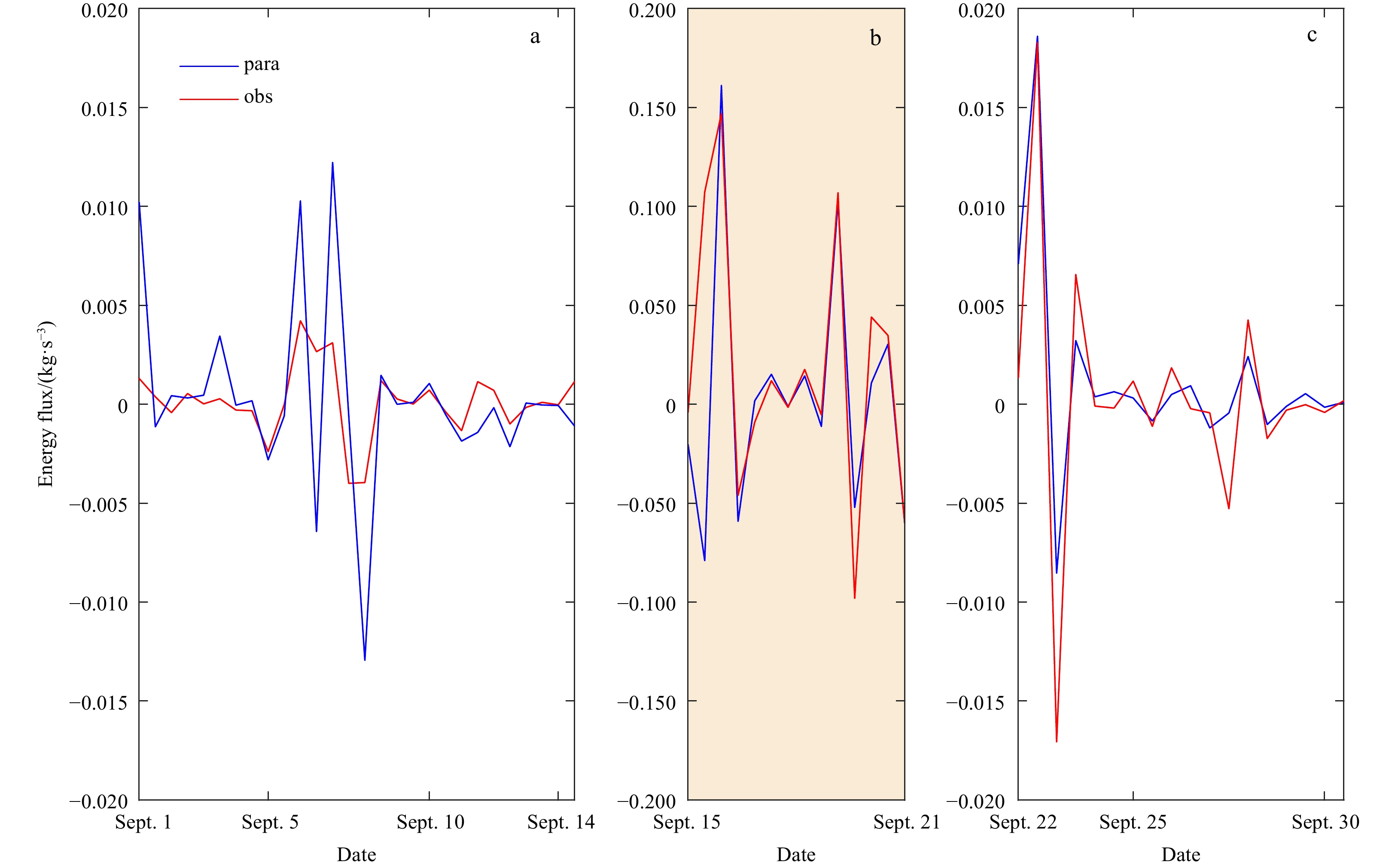
Figure 3. Near-inertial energy input from winds into the ocean estimated with the observations (
${E}_{{\rm{obs}}}^{i} = {\vec{{{u}}}}_{{\rm{obs}}}^{i} \cdot \vec{{{{{\tau}}}} }$ ; red lines) and the J13 scheme (${E}_{{\rm{para}}}^{i} = {\vec{{{u}}}}_{{\rm{para}}}^{i} \cdot \vec{{{\tau}} }$ ; blue lines). See the main text for details. All data are obtained from Buoy #2. Since the energy input is much larger during typhoon, the vertical scale for b is different from the vertical scales for a and c.
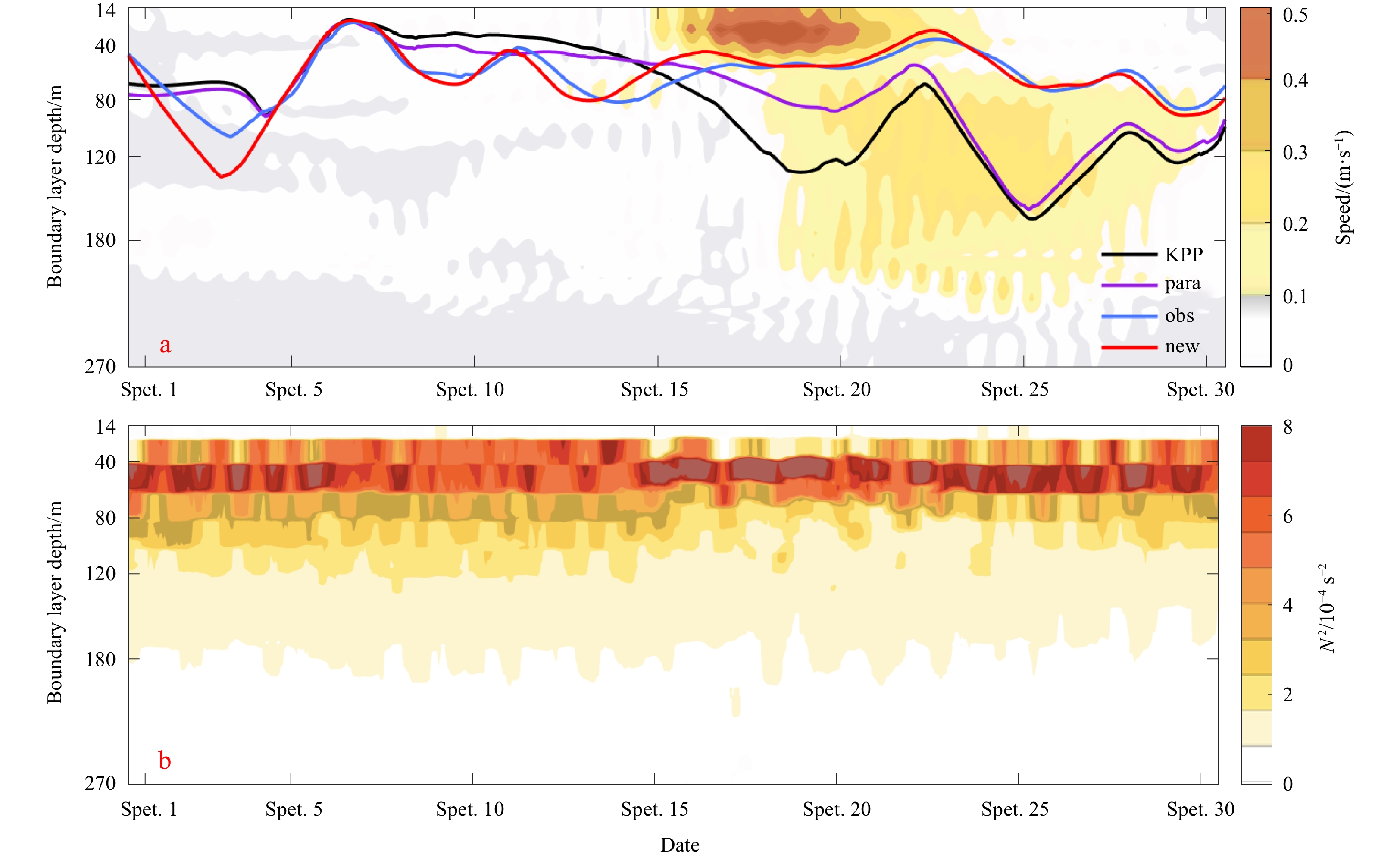
Figure 4. The comparison of the boundary layer depth. a. Colors denote the speeds of near-inertial currents at Buoy #2, which are obtained with a Butterworth bandpass filter between 0.7f and 1.3f. The blue line shows the boundary layer depth
$ {h}_{{\rm{obs}}} $ obtained following the classical KPP scheme (Eq. (21) in Large et al. (1994)). The black line shows$ {h}_{{\rm{KPP}}}^{n} $ in Eq. (5), the purple line shows$ {h}_{{\rm{para}}} $ in Eq. (6), and the red line shows$ {h}_{{\rm{para}}\_{\rm{new}}} $ in Eq. (11). b. The buoyancy frequency$ {N}^{2} $ at Buoy #2. All data are smoothed with a 12-hour running mean. Para: parameterization, obs: observation.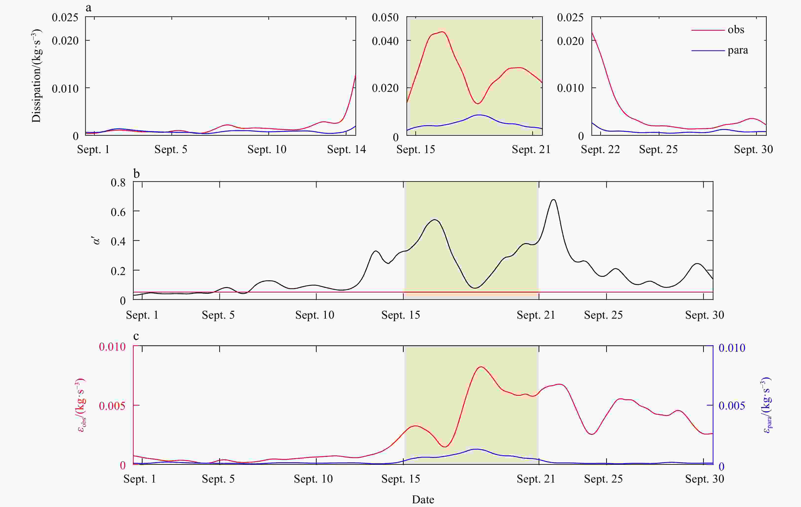
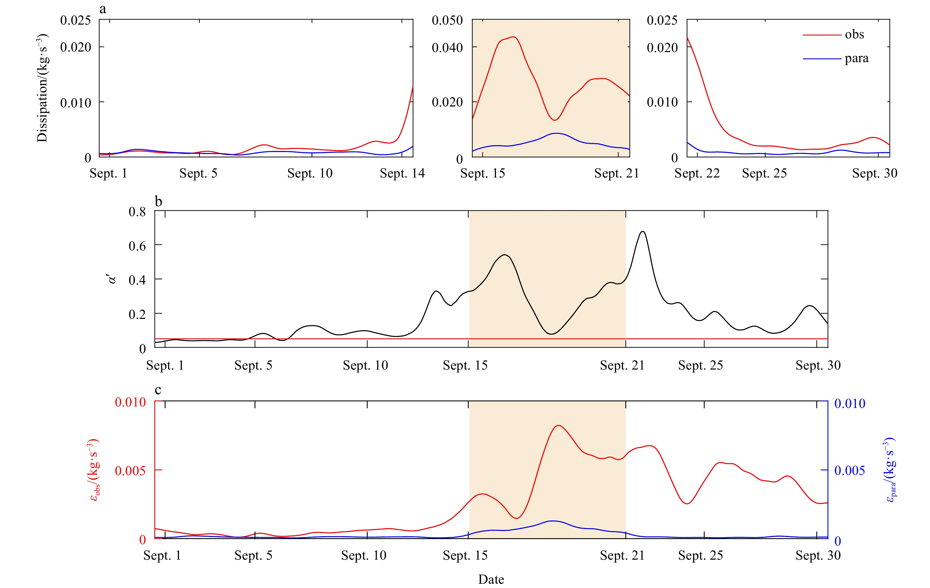
Figure 5. The comparison of near-inertial energy dissipation. a. Near-inertial energy dissipation in the upper boundary layer estimated with observations (
${\varepsilon}_{{\rm{obs}}}^{i}$ , red line) and with the J13 scheme ($\varepsilon_{{\rm{para}}}^{{i}}$ , blue line) at Buoy #2. b.$ {\alpha }{{'}}=\mathrm{\Delta }{K}_{h}^{i}/\mathrm{\Delta }{K}_{h} $ , which indicates the ratio between the energy dissipation associated with the NIWs and the total energy dissipation in the upper boundary layer; the red line shows the ratio of 0.05, which is used in the J13 scheme. c. Near-inertial energy dissipation below the upper boundary layer estimated with observations ($\varepsilon_{{\rm{obs}}}$ , red line) and with the J13 scheme ($\varepsilon_{{\rm{para}}}$ , blue line) at Buoy #2. See the main text for the detailed methods to estimate the energy dissipation.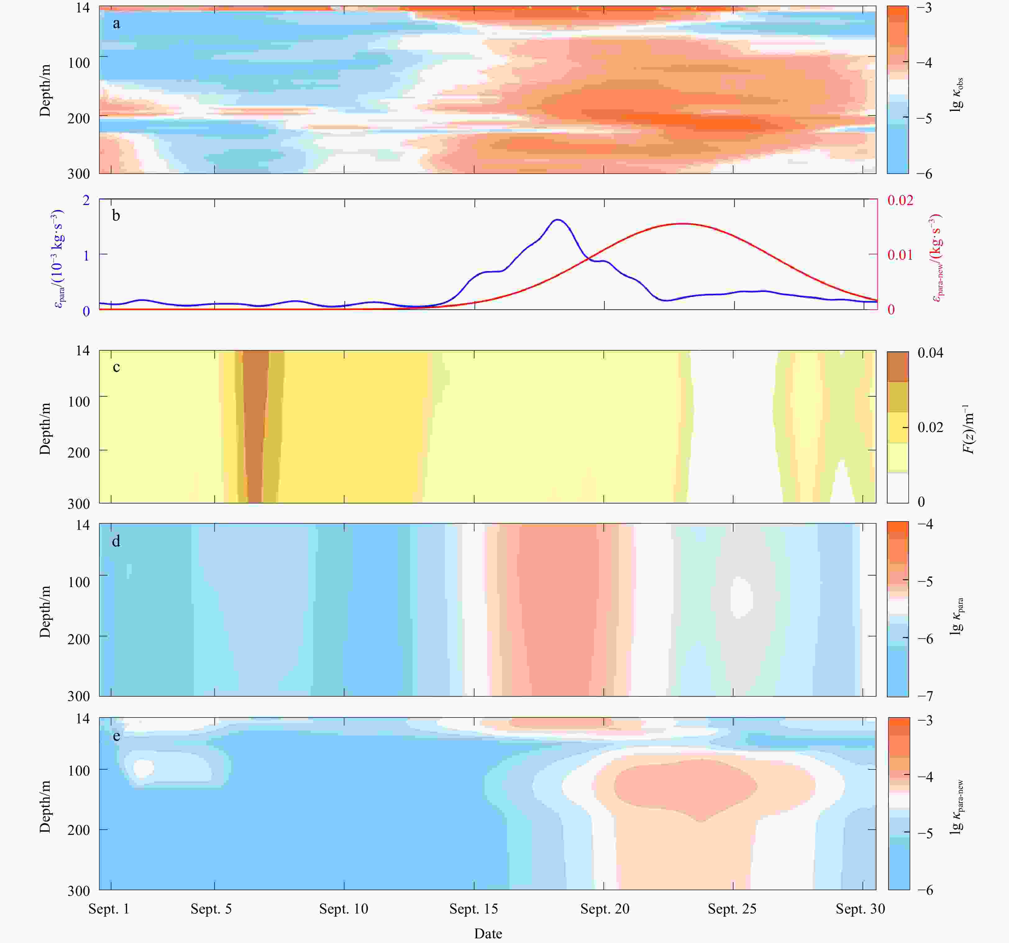
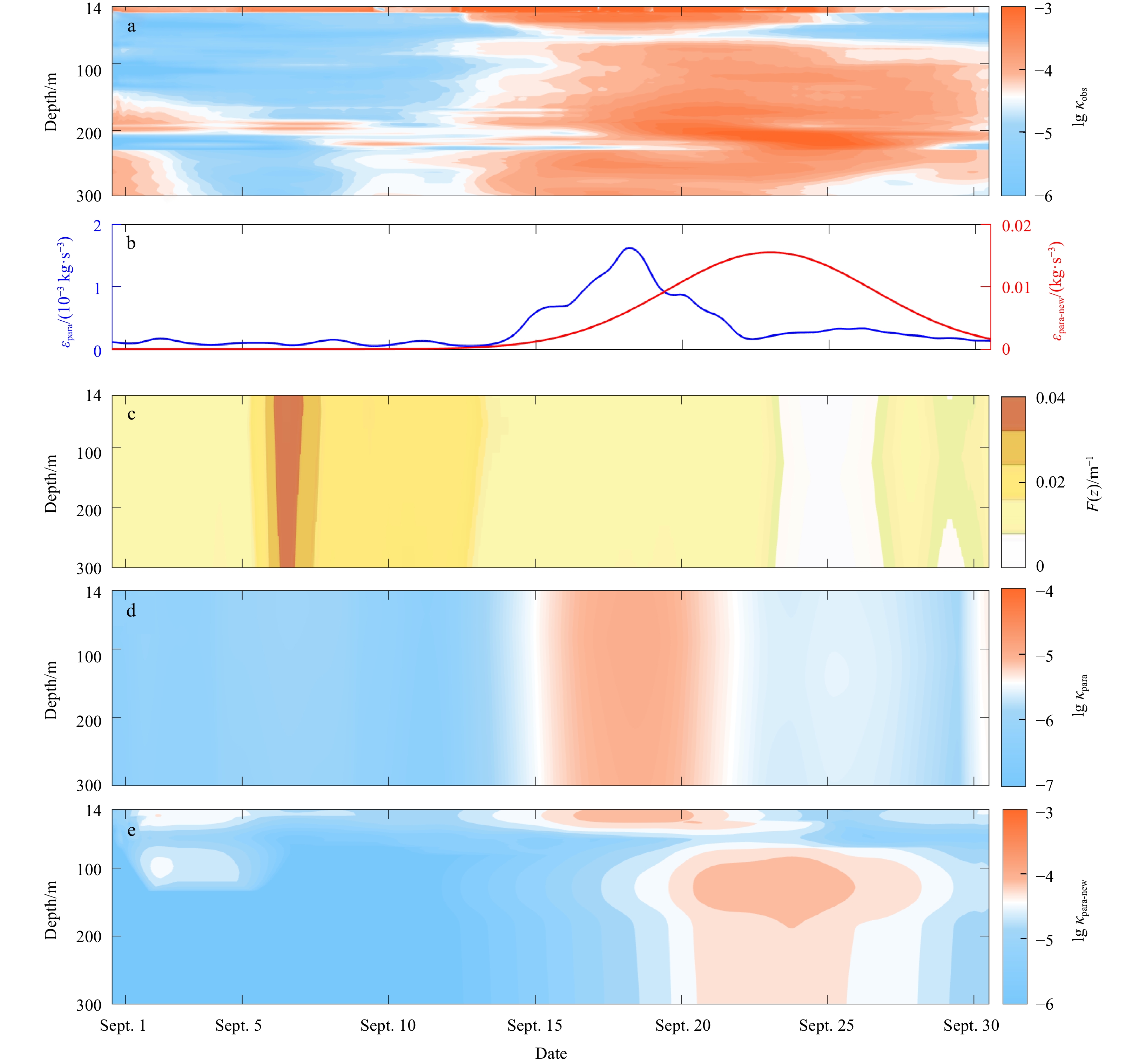
Figure 6. The comparison of diffusivities. a. Vertical profiles of
$\rm{l}\rm{g}\,{\kappa }_{{\rm{obs}}}$ at Buoy #2, where${\kappa }_{{\rm{obs}}}={\varGamma }\dfrac{\varepsilon_{{\rm{obs}}}\left(z\right)}{{{\rho }{N}}^{2}}$ is the diffusivity. b.$ \varepsilon_{{\rm{para}}} $ (blue line) in Eq. (7) and$\varepsilon_{{\rm{para}}\_{\rm{new}}}$ (red line) in Eq. (12) at Buoy #2. c. Vertical profiles of$F \left(z\right)$ at Buoy #2. The boundary layer depth (h) in$F \left(z\right)$ is set to${h}_{{\rm{para}}}$ (Eq. (6) and purple line in Fig. 4a). d. Vertical profiles of$\mathrm{l}\mathrm{g}\,{\kappa }_{{\rm{para}}}$ . e. Vertical profiles of$\mathrm{l}\mathrm{g}\,{\kappa }_{{\rm{para}}\_{\rm{new}}}$ . The unit for all diffusivities is m2 /s.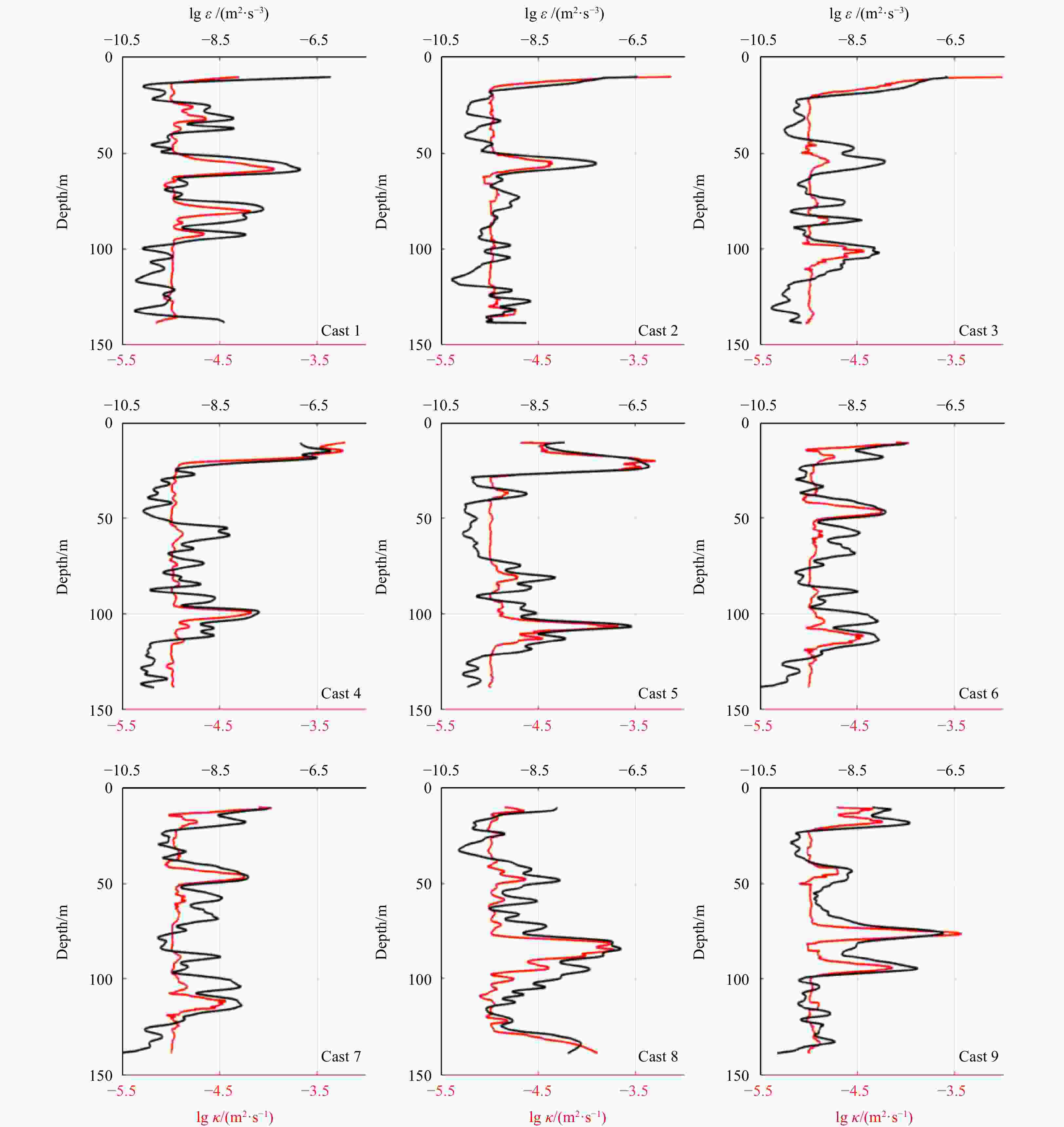
Figure 7.
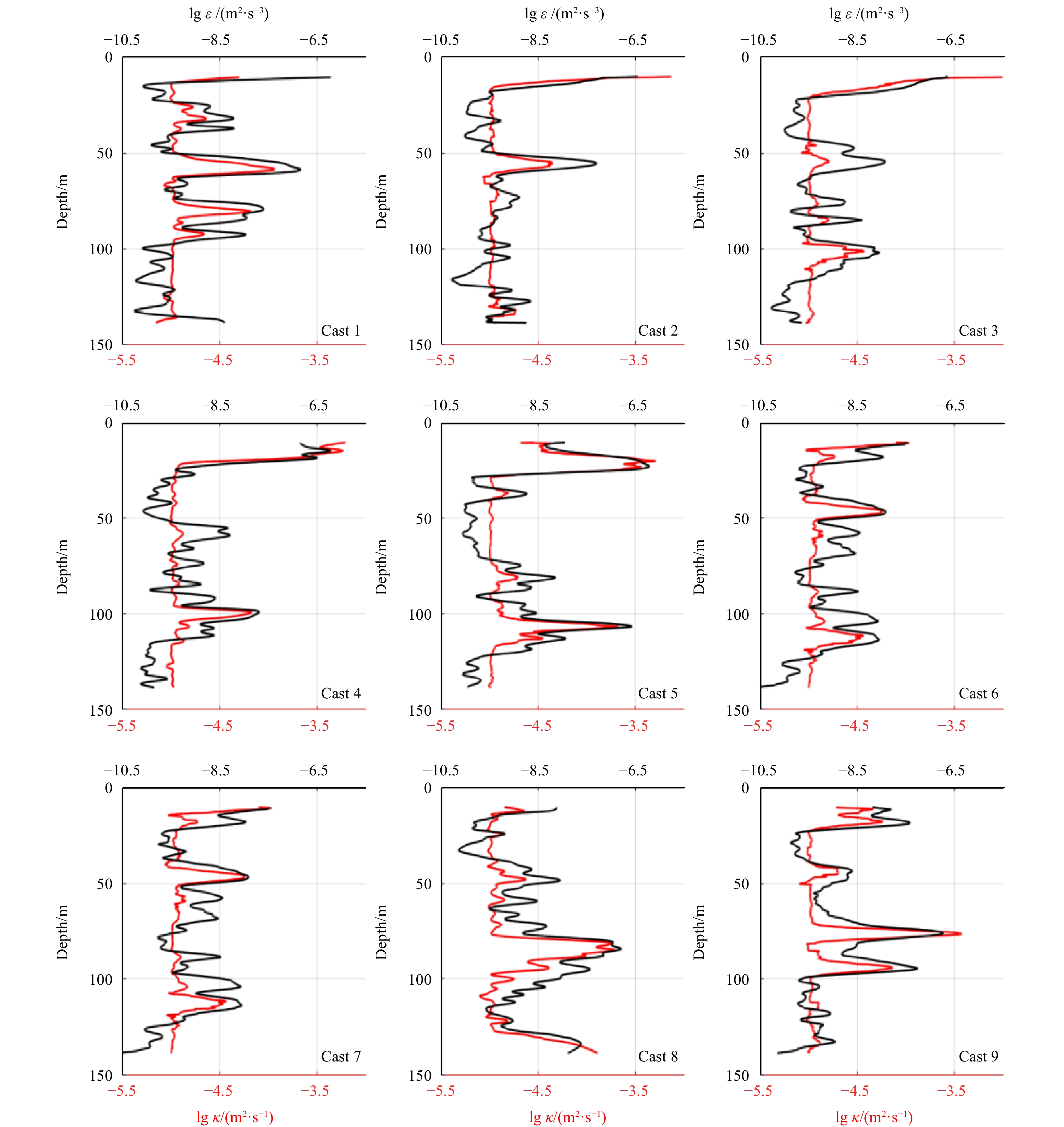
$\mathrm{l}\mathrm{g}\,\varepsilon$ and$\mathrm{l}\mathrm{g}\, \kappa$ of nine casts. Black lines show$\mathrm{l}\mathrm{g}\,\varepsilon$ , where ε is the turbulent kinetic energy dissipation rate and is computed by the shear spectra that are observed by the VMP-250 in the SCS in 2019. Red lines show corresponding$\mathrm{l}\mathrm{g}\,\kappa$ , where$\kappa = \frac{{\varGamma }\varepsilon }{{N}^{2}}$ is the diffusivities.
Figure 8. The comparison of the vertical structure function and the mean diffusivity. a. Vertical profiles of
$ {{F}}_{{\rm{new}}}\left(z\right) $ (blue line) and F(z) (black line) at Buoy #2. b. Time average$\mathrm{l}\mathrm{g}\,{\kappa }_{{\rm{obs}}}$ (red line),$\mathrm{l}\mathrm{g}\,{\kappa }_{{\rm{para}}}$ (black line) and$\mathrm{l}\mathrm{g}\,{\kappa }_{{\rm{para}}\_{\rm{new}}}$ (blue line) from September 14 to 30. The unit for all diffusivities is m2/s.Table 1. Locations of the buoys deployed in the South China Sea in 2014
Buoy ID Latitude Longitude 1 19.70°N 116.00°E 2 18.20°N 115.50°E 3 18.70°N 116.50°E 4 19.20°N 117.50°E 5 17.70°N 117.00°E Note: The locations are also marked in Fig. 1.  下载: 导出CSV
Table 2. Definitions of key variables
Variable Definition Variable Definition u, v zonal and meridional ocean current velocities in observations $ {\varepsilon}_{{\rm{para}}}^{i} $ energy dissipation due to NIWs in the boundary layer in the J13 scheme $ {u}_{{\rm{para}}}^{i} $, $ {v}_{{\rm{para}}}^{i} $ near-inertial velocities in the J13 scheme $ {\varepsilon}_{{\rm{obs}}}^{i} $ energy dissipation due to NIWs in the boundary layer in observations $ {u}_{{\rm{obs}}}^{i} $, $ {v}_{{\rm{obs}}}^{i} $ near-inertial velocities in observations $ {\varepsilon}_{{\rm{para}}\_{\rm{new}}}^{i} $ energy dissipation due to NIWs in the boundary layer in modified scheme $ {u}_{1}^{n} $, $ {v}_{1}^{n} $ velocities without NIWs at the sea surface $ {\varepsilon}_{{\rm{para}}} $ near-inertial energy input available for mixing below the boundary layer in the J13 scheme $ {u}_{1}^{i} $, $ {v}_{1}^{i} $ near-inertial velocities at the sea surface $ {\varepsilon}_{{\rm{obs}}} $ near-inertial energy input available for mixing below the boundary layer in observations $ {u}_{h}^{n} $, $ {v}_{h}^{n} $ velocities without NIWs at the boundary layer depth $ {\varepsilon}_{{\rm{para}}\_{\rm{new}}} $ near-inertial energy input available for mixing below the boundary layer in modified scheme $ {u}_{h}^{i} $, $ {v}_{h}^{i} $ near-inertial velocities at the boundary layer depth $ {\kappa }_{{\rm{para}}} $ diffusivity due to NIWs in the J13 scheme $ {h}_{{\rm{para}}} $ boundary layer depth in the J13 scheme $ {\kappa }_{{\rm{obs}}} $ diffusivity due to NIWs in observations $ {h}_{{\rm{obs}}} $ boundary layer depth in observations $ {\kappa }_{{\rm{para}}\_{\rm{new}}} $ diffusivity due to NIWs in modified scheme $ {h}_{{\rm{para}}\_{\rm{new}}} $ boundary layer depth in modified scheme
下载: 导出CSV
-
Alford M H. 2020. Revisiting near-inertial wind work: slab models, relative stress, and mixed layer deepening. Journal of Physical Oceanography, 50(11): 3141–3156. doi: 10.1175/JPO-D-20-0105.1 Alford M H, Cronin M F, Klymak J M. 2012. Annual cycle and depth penetration of wind-generated near-inertial internal waves at ocean station papa in the Northeast Pacific. Journal of Physical Oceanography, 42(6): 889–909. doi: 10.1175/JPO-D-11-092.1 Alford M H, Gregg M C. 2001. Near-inertial mixing: Modulation of shear, strain and microstructure at low latitude. Journal of Geophysical Research: Oceans, 106(C8): 16947–16968. doi: 10.1029/2000JC000370 Alford M H, MacKinnon J A, Simmons H L, et al. 2016. Near-inertial internal gravity waves in the ocean. Annual Review of Marine Science, 8: 95–123. doi: 10.1146/annurev-marine-010814-015746 Alford M H, Whitmont M. 2007. Seasonal and spatial variability of near-inertial kinetic energy from historical moored velocity records. Journal of Physical Oceanography, 37(8): 2022–2037. doi: 10.1175/JPO3106.1 Chen Gengxin, Xue Huijie, Wang Dongxiao, et al. 2013. Observed near-inertial kinetic energy in the northwestern South China Sea. Journal of Geophysical Research: Oceans, 118(10): 4965–4977. doi: 10.1002/jgrc.20371 D’Asaro E A. 1985. The energy flux from the wind to near-inertial motions in the surface mixed layer. Journal of Physical Oceanography, 15(8): 1043–1059. doi: 10.1175/1520-0485(1985)015<1043:TEFFTW>2.0.CO;2 D’Asaro E A. 1995. A collection of papers on the ocean storms experiment. Journal of Physical Oceanography, 25(11): 2817–2818. doi: 10.1175/1520-0485(1995)025<2817:ACOPOT>2.0.CO;2 D’Asaro E A, Black P G, Centurioni L R, et al. 2014. Impact of typhoons on the ocean in the Pacific. Bulletin of the American Meteorological Society, 95(9): 1405–1418. doi: 10.1175/BAMS-D-12-00104.1 D’Asaro E A, Eriksen C C, Levine M D, et al. 1995. Upper-ocean inertial currents forced by a strong storm. Part I: Data and comparisons with linear theory. Journal of Physical Oceanography, 25(11): 2909–2936. doi: 10.1175/1520-0485(1995)025<2909:UOICFB>2.0.CO;2 Fedorov A V, Brierley C M, Emanuel K. 2010. Tropical cyclones and permanent El Niño in the early Pliocene epoch. Nature, 463(7284): 1066–1070. doi: 10.1038/nature08831 Fleagle R G, Businger J A. 1980. An Introduction to Atmospheric Physics. New York, NY, USA: Academic Press Fu L L. 1981. Observations and models of inertial waves in the deep ocean. Reviews of Geophysics, 19(1): 141–170. doi: 10.1029/RG019i001p00141 Furuichi N, Hibiya T, Niwa Y. 2008. Model-predicted distribution of wind-induced internal wave energy in the world’s oceans. Journal of Geophysical Research: Oceans, 113: C09034 Hebert D, Moum J N. 1994. Decay of a near-inertial wave. Journal of Physical Oceanography, 24(11): 2334–2351. doi: 10.1175/1520-0485(1994)024<2334:DOANIW>2.0.CO;2 Jaimes B, Shay L K. 2010. Near-inertial wave wake of Hurricanes Katrina and Rita over mesoscale oceanic eddies. Journal of Physical Oceanography, 40(6): 1320–1337. doi: 10.1175/2010JPO4309.1 Jochum M, Briegleb B P, Danabasoglu G, et al. 2013. The impact of oceanic near-inertial waves on climate. Journal of Climate, 26(9): 2833–2844. doi: 10.1175/JCLI-D-12-00181.1 Knutson T R, McBride J L, Chan J, et al. 2010. Tropical cyclones and climate change. Nature Geoscience, 3(3): 157–163. doi: 10.1038/ngeo779 Kunze E, Briscoe M G, Williams A J III. 1990. Interpreting shear and strain fine structure from a neutrally buoyant float. Journal of Geophysical Research: Oceans, 95(C10): 18111–18125. doi: 10.1029/JC095iC10p18111 Kunze E, Sanford T B. 1984. Observations of near-inertial waves in a front. Journal of Physical Oceanography, 14(3): 566–581. doi: 10.1175/1520-0485(1984)014<0566:OONIWI>2.0.CO;2 Large W G, Grawford G B. 1995. Observations and simulations of upper-ocean response to wind events during the Ocean Storms Experiment. Journal of Physical Oceanography, 25(11): 2831–2852. doi: 10.1175/1520-0485(1995)025<2831:OASOUO>2.0.CO;2 Large W G, McWilliams J C, Doney S C. 1994. Oceanic vertical mixing: A review and a model with a nonlocal boundary layer parameterization. Reviews of Geophysics, 32(4): 363–403. doi: 10.1029/94RG01872 Levine M D, Zervakis V. 1995. Near-inertial wave propagation into the pycnocline during ocean storms: observations and model comparison. Journal of Physical Oceanography, 25(11): 2890–2908. doi: 10.1175/1520-0485(1995)025<2890:NIWPIT>2.0.CO;2 Li Xinming, Qian Qingying. 1989. The wind stress field over the South China Sea. Journal of Ocean University of Qingdao, 19(3): 10–18 MacKinnon J A, Zhao Zhongxiang, Whalen C B, et al. 2017. Climate process team on internal wave-driven ocean mixing. Bulletin of the American Meteorological Society, 98(11): 2429–2454. doi: 10.1175/BAMS-D-16-0030.1 Munk W, Wunsch C. 1998. Abyssal recipes II: energetics of tidal and wind mixing. Deep-Sea Research Part I: Oceanographic Research Papers, 45(12): 1977–2010. doi: 10.1016/S0967-0637(98)00070-3 Olbers D, Eden C. 2013. A global model for the diapycnal diffusivity induced by internal gravity waves. Journal of Physical Oceanography, 43(8): 1759–1779. doi: 10.1175/JPO-D-12-0207.1 Osborn T R. 1980. Estimates of the local rate of vertical diffusion from dissipation measurements. Journal of Physical Oceanography, 10(1): 83–89. doi: 10.1175/1520-0485(1980)010<0083:EOTLRO>2.0.CO;2 Park J J, Kim K, Schmitt R W. 2009. Global distribution of the decay timescale of mixed layer inertial motions observed by satellite-tracked drifters. Journal of Geophysical Research, 114(C11): C11010. doi: 10.1029/2008JC005216 Pedlowsky J, Miles J W. 2004. Waves in the ocean and atmosphere: Introduction to wave dynamics. Applied Mechanics Reviews, 57(4): B20 Price J F. 1981. Upper ocean response to a hurricane. Journal of Physical Oceanography, 11(2): 153–175. doi: 10.1175/1520-0485(1981)011<0153:UORTAH>2.0.CO;2 Qi Hongbo, De Szoeke R A, Paulson C A, et al. 1995. The structure of near-inertial waves during ocean storms. Journal of Physical Oceanography, 25(11): 2853–2871. doi: 10.1175/1520-0485(1995)025<2853:TSONIW>2.0.CO;2 Sanford T B, Price J F, Girton J B. 2011. Upper-ocean response to Hurricane Frances (2004) observed by profiling EM-APEX floats. Journal of Physical Oceanography, 41(6): 1041–1056. doi: 10.1175/2010JPO4313.1 Silverthorne K E, Toole J M. 2009. Seasonal kinetic energy variability of near-inertial motions. Journal of Physical Oceanography, 39(4): 1035–1049. doi: 10.1175/2008JPO3920.1 Simmons H L, Alford M H. 2012. Simulating the long-range swell of internal waves generated by ocean storms. Oceanography, 25(2): 30–41. doi: 10.5670/oceanog.2012.39 Sloyan B M, Rintoul S R. 2001. The southern ocean limb of the global deep overturning circulation. Journal of Physical Oceanography, 31(1): 143–173. doi: 10.1175/1520-0485(2001)031<0143:TSOLOT>2.0.CO;2 Ten Doeschate A, Sutherland G, Esters L, et al. 2017. ASIP: profiling the upper ocean. Oceanography, 30(2): 33–35. doi: 10.5670/oceanog.2017.216 Troen I, Petersen E L. 1989. European Wind Atlas. Roskilde, Denmark: Risø National Laboratory van Haren H, Gostiaux L. 2012. Energy release through internal wave breaking. Oceanography, 25(2): 124–131. doi: 10.5670/oceanog.2012.47 Wang Wei, Huang Rui Xin. 2004. Wind energy input to the Ekman layer. Journal of Physical Oceanography, 34(5): 1267–1275. doi: 10.1175/1520-0485(2004)034<1267:WEITTE>2.0.CO;2 Watanabe M, Hibiya T. 2002. Global estimates of the wind-induced energy flux to inertial motions in the surface mixed layer. Geophysical Research Letters, 29(8): 64-1–64-3 Webster F. 1968. Observations of inertial-period motions in the deep sea. Reviews of Geophysics, 6(4): 473–490. doi: 10.1029/RG006i004p00473 Wolk F, Yamazaki H, Seuront L, et al. 2002. A new free-fall profiler for measuring biophysical microstructure. Journal of Atmospheric and Oceanic Technology, 19(5): 780–793. doi: 10.1175/1520-0426(2002)019<0780:ANFFPF>2.0.CO;2 Wunsch C, Ferrari R. 2004. Vertical mixing, energy, and the general circulation of the oceans. Annual Review of Fluid Mechanics, 36: 281–314. doi: 10.1146/annurev.fluid.36.050802.122121 Ying Ming, Zhang Wei, Yu Hui, et al. 2014. An overview of the China meteorological administration tropical cyclone database. Journal of Atmospheric and Oceanic Technology, 31(2): 287–301. doi: 10.1175/JTECH-D-12-00119.1 Zhai Xiaoming, Greatbatch R J, Eden C. 2007. Spreading of near-inertial energy in a 1/12° model of the North Atlantic Ocean. Geophysical Research Letters, 34(10): L10609. doi: 10.1029/2007GL029895 Zhang Han, Chen Dake, Zhou Lei, et al. 2016. Upper ocean response to typhoon Kalmaegi (2014). Journal of Geophysical Research: Oceans, 121(8): 6520–6535. doi: 10.1002/2016JC012064 Zhang Han, Wu Renhao, Chen Dake, et al. 2018. Net modulation of upper ocean thermal structure by Typhoon Kalmaegi (2014). Journal of Geophysical Research: Oceans, 123(10): 7154–7171. doi: 10.1029/2018JC014119 Zhang Yu, Zhang Zhengguang, Chen Dake, et al. 2020. Strengthening of the Kuroshio current by intensifying tropical cyclones. Science, 368(6494): 988–993. doi: 10.1126/science.aax5758 -


 点击查看大图

计量
- 文章访问数: 359
- HTML全文浏览量: 111
- PDF下载量: 26
- 被引次数: 0