

Circulation in the South China Sea is in a state of forced oscillation: Results from a simple reduced gravity model with a closed boundary
-
Abstract:
The South China Sea (SCS) is a narrow semi-enclosed basin, ranging from 4°–6°N to 21°–22°N meridionally. It is forced by a strong annual cycle of monsoon-related wind stress. The Coriolis parameter f increases at least three times from the southern basin to the northern basin. As a result, the basin-cross time for the first baroclinic Rossby wave in the southern part of the basin is about 10-times faster than that in the northern part, which plays the most vitally important role in setting the circulation. At the northernmost edge of SCS, the first baroclinic Rossby wave takes slightly less than 1 year to move across the basin, however, it takes only 1–2 months in the southernmost part. Therefore, circulation properties for a station in the model ocean are not solely determined by the forcing at that time instance only; instead, they depend on the information over the past months. The combination of a strong annual cycle of wind forcing and large difference of basin-cross time for the first baroclinic Rossby wave leads to a strong seasonal cycle of the circulation in the SCS, hence, the circulation is dominated by the forced oscillations, rather than the quasi-steady state discussed in many textbooks.The circulation in the SCS is explored in detail by using a simple reduced gravity model forced by seasonally varying zonal wind stress. In particular, for a given time snap the western boundary current in the SCS cannot play the role of balancing mass transport across each latitude nor balancing mechanical energy and vorticity in the whole basin. In a departure from the steady wind-driven circulation discussed in many existing textbooks, the circulation in the SCS is characterized by the imbalance of mechanical energy and vorticity for the whole basin at any part of the seasonal cycle. In particular, the western boundary current in the SCS cannot balance the mass, mechanical energy, and vorticity in the seasonal cycle of the basin. Consequently, the circulation near the western boundary cannot be interpreted in terms of the wind stress and thermohaline forcing at the same time. Instead, circulation properties near the western boundary should be interpreted in terms of the contributions due to the delayed wind stress and the eastern boundary layer thickness. In fact, there is a clear annual cycle of net imbalance of mechanical energy and vorticity source/sink. Results from such a simple model may have important implications for our understanding of the complicated phenomena in the SCS, either from in-situ observations or numerical simulations. -
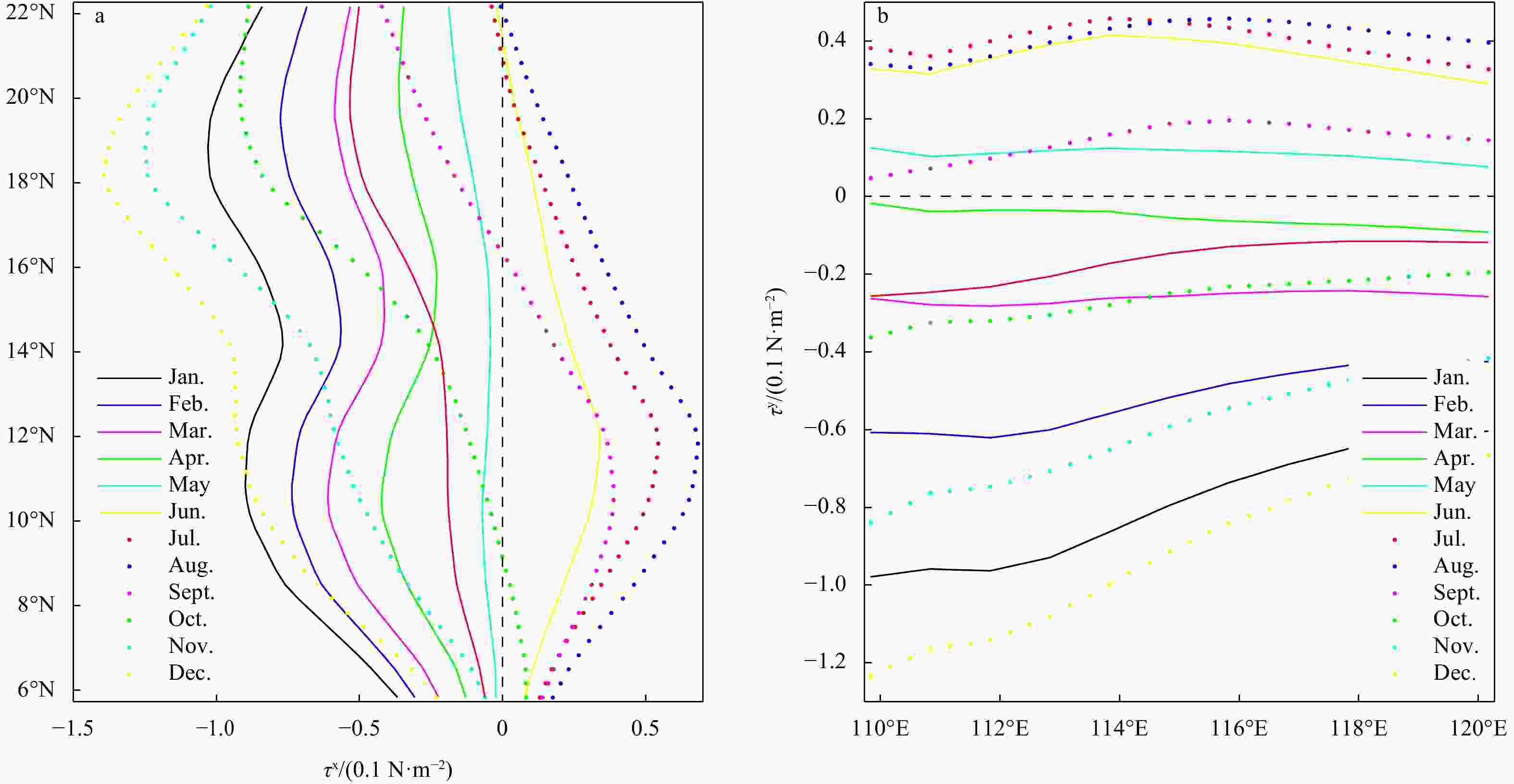
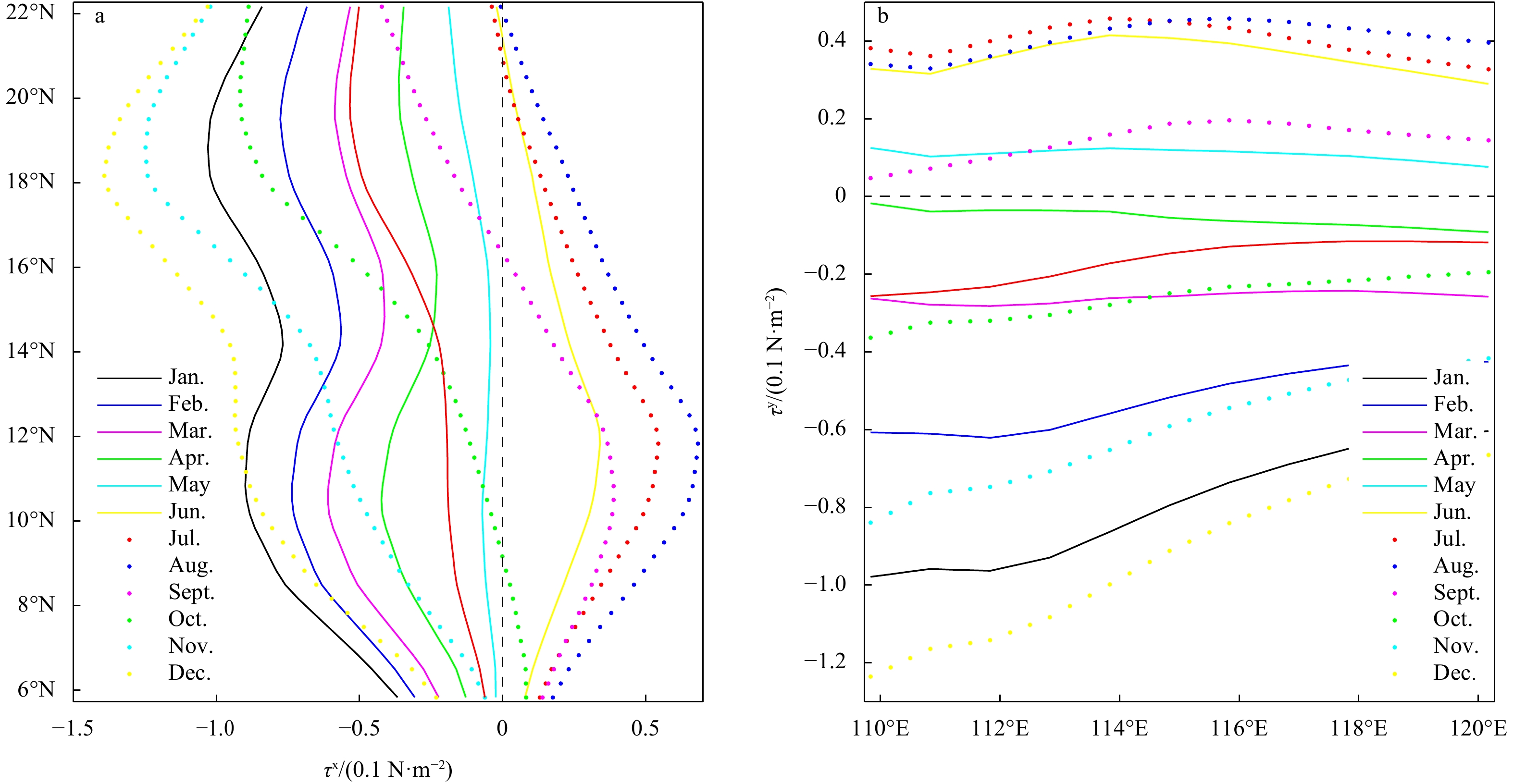
Figure 1. Idealized monthly mean wind stress for the model. a. Zonal wind (independent of longitude); b. meridional wind (independent of latitude); based on Global Ocean Data Assimilation System data.
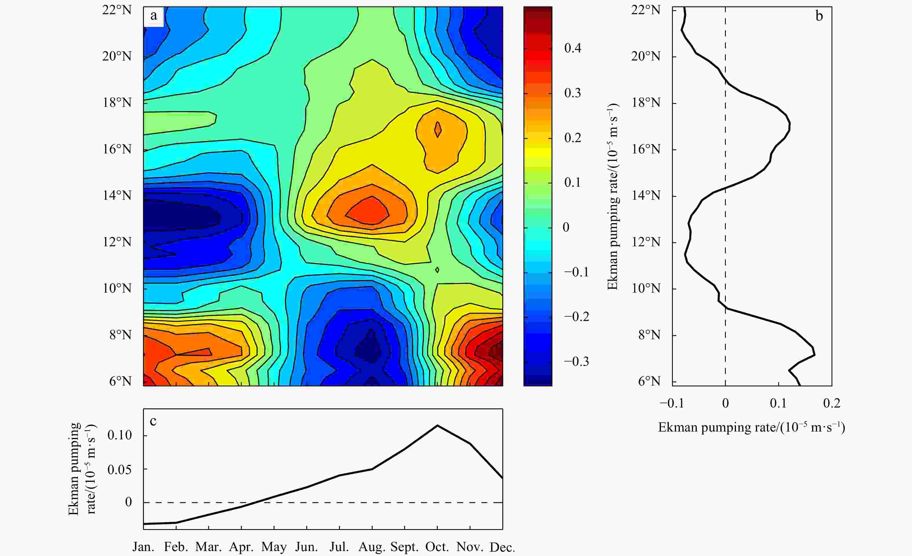
Figure 2. The time-latitude diagram of the climatological monthly mean Ekman pumping rate for the model forced by the zonally mean zonal wind stress only (a); the annual mean Ekman pumping rate (b); the basin mean Ekman pumping rate (c).
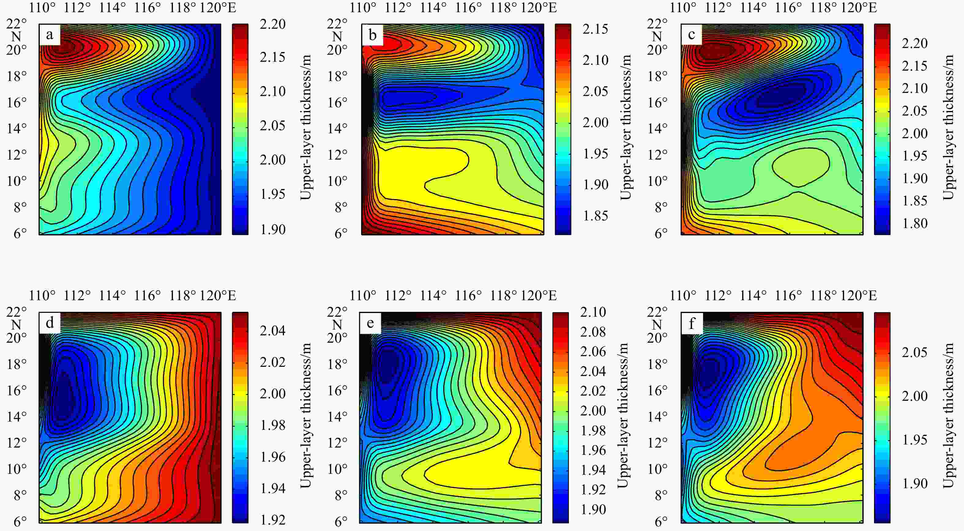
Figure 3. Layer depth in January (a−c) and July (d−f) for the simple model forced by zonally mean zonal wind (a, d, Exp. 1), by zonally mean zonal wind and meridionally mean meridional wind (b, e , Exp. 2) and 2D wind (c, f , Exp. 3).
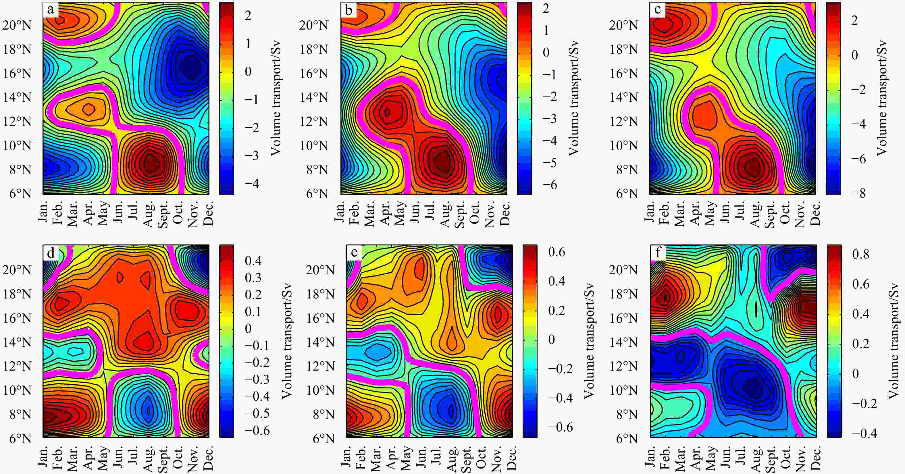
Figure 4. Western boundary current transport (a−c) and eastern boundary current (d−f) for a simple model forced by zonally mean zonal wind (a, d, Exp. 1), by zonally mean zonal wind and meridionally mean meridional wind (b, e, Exp. 2) and 2D wind (c, f, Exp. 3). The magenta curves indicate the zero contours (1 Sv=106 m3/s).
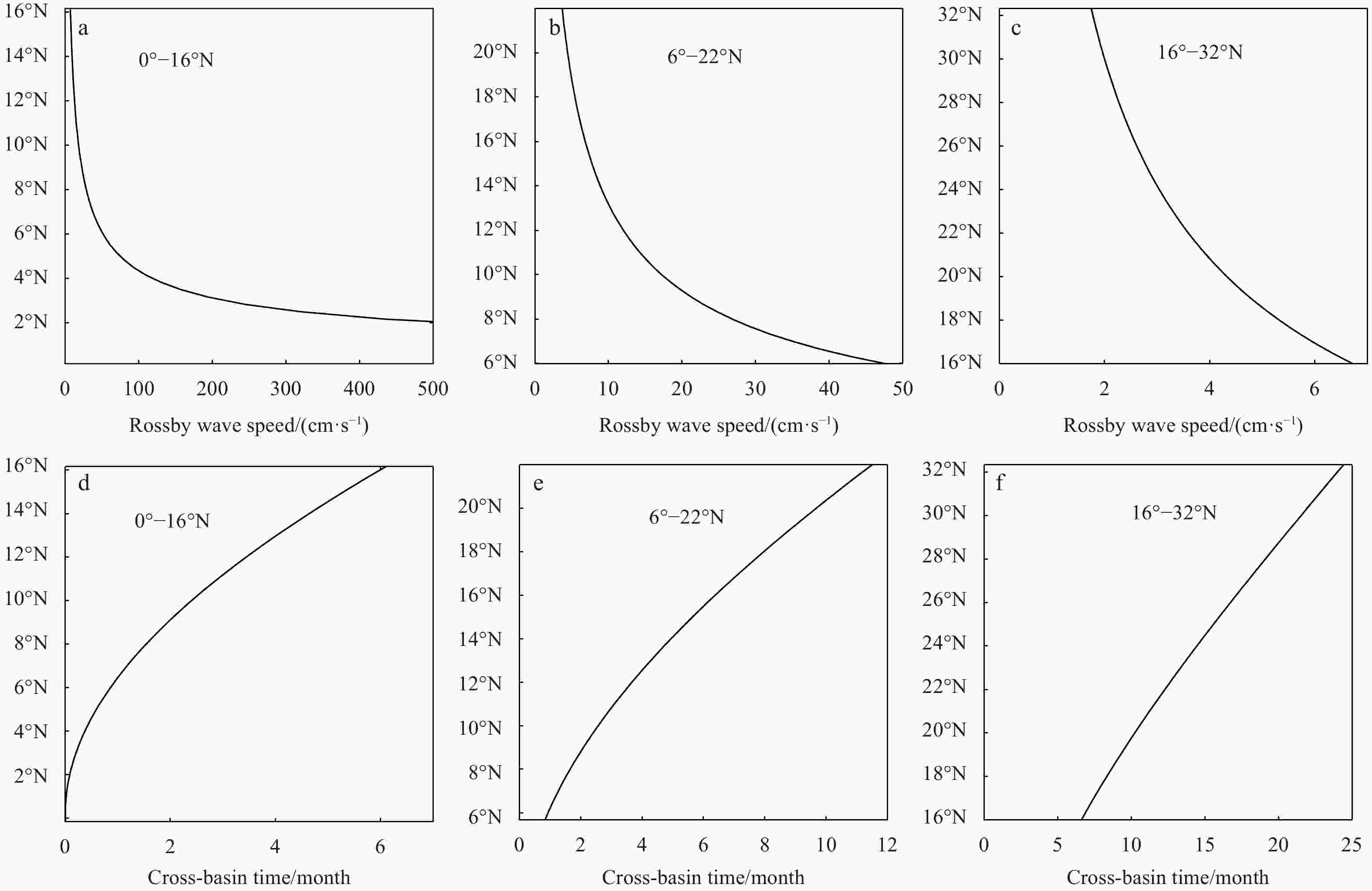
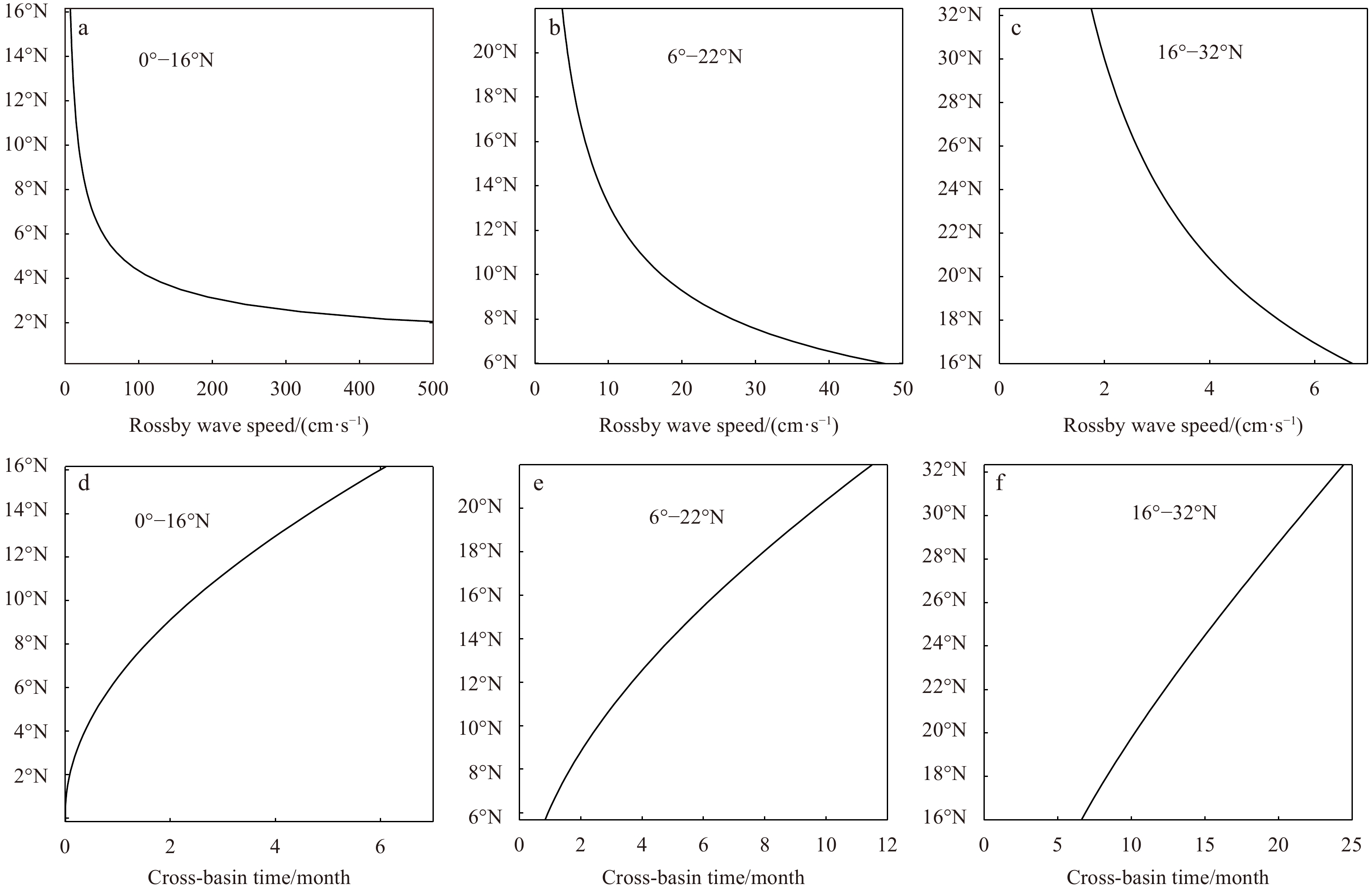
Figure 5. Rossby wave speed (a−c) and the cross-basin time (d−f) for the model located between 0°–16°N (Exp. 4, a, d); the model located between 6°–22°N for Exp. 1 (b, e) and the model located between 16°–32°N for Exp. 5 (c, f).
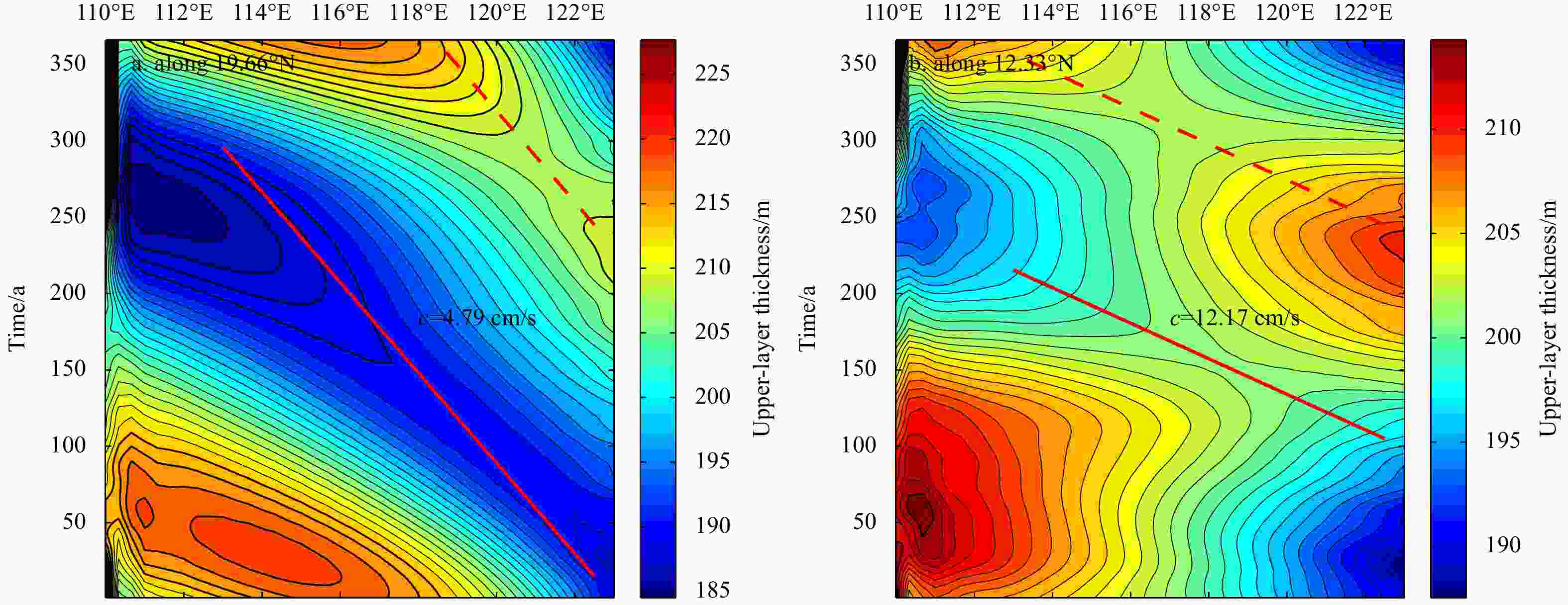
Figure 6. Time evolution of layer depth for the model forced by zonal wind stress only (Exp. 1). The dashed and solid red lines indicate the corresponding signal speed.
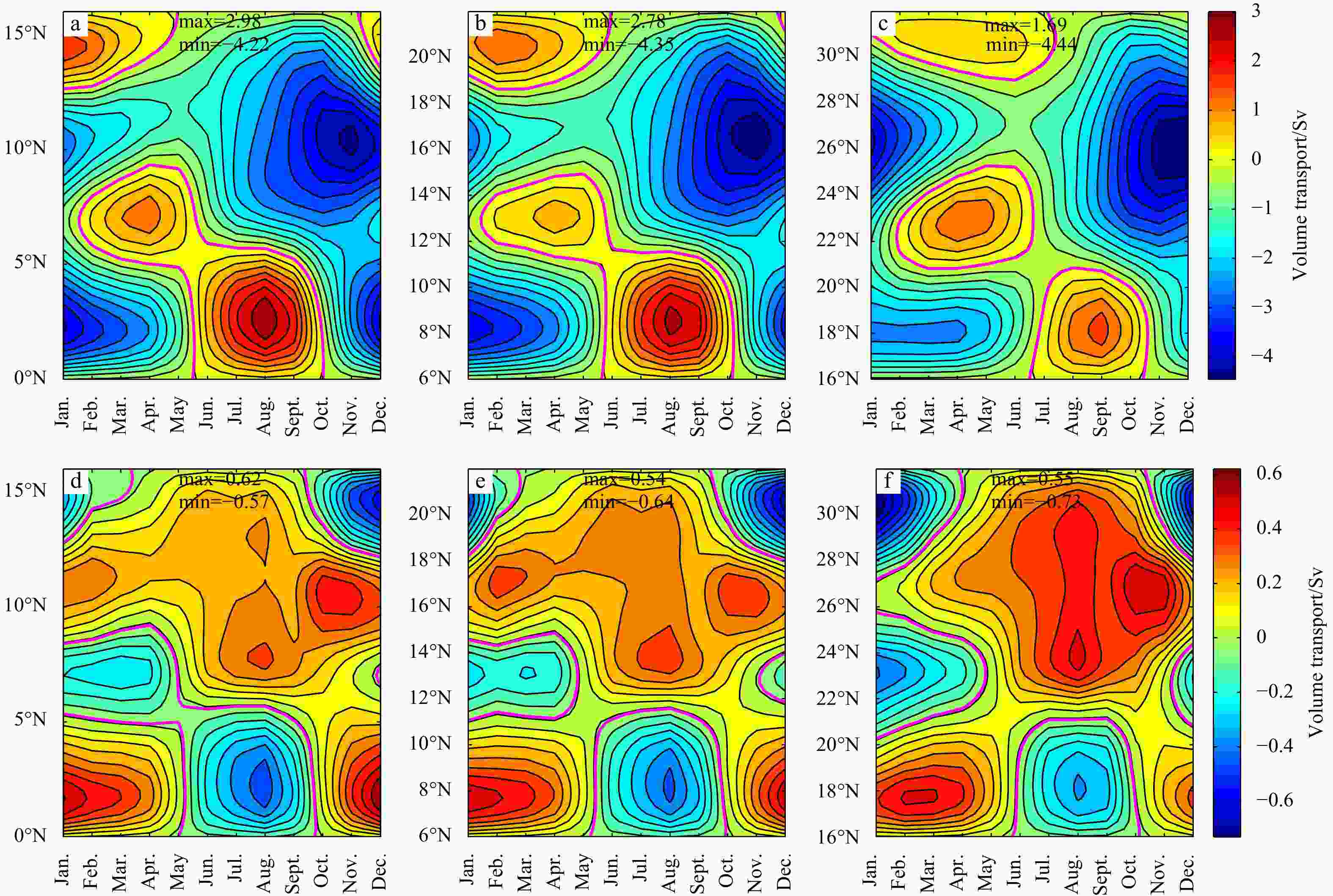
Figure 7. Volumetric transport of the western boundary current (a−c) and eastern boundary current (d−f). Left column for the model located between 0°–16°N (Exp. 4); middle column for the model located between 6°–22°N (Exp. 1); right column for the model located between 16°–32°N (Exp. 5). The magenta curves indicate the zero contours (1 Sv=106 m3/s).

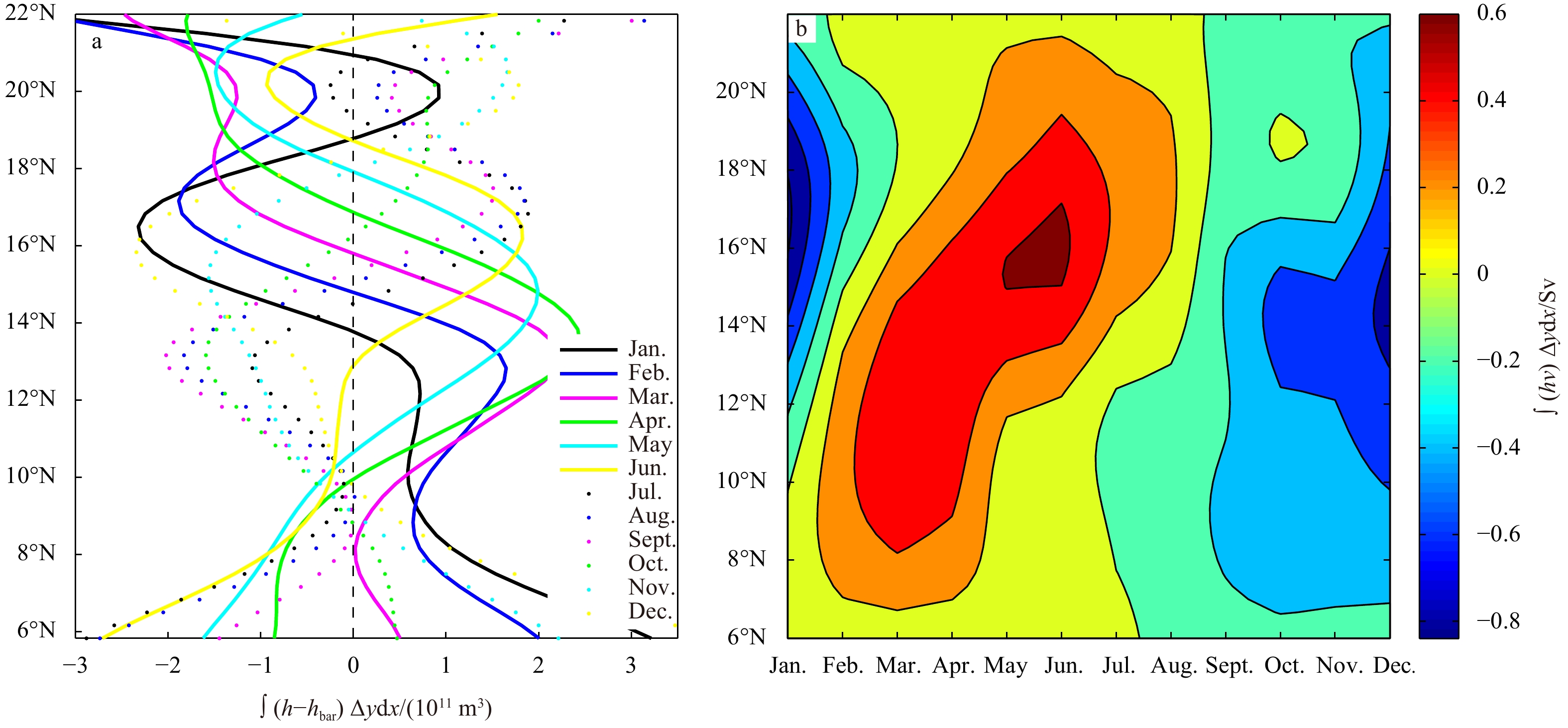
Figure 8. Experiments forced by idealized monthly zonal/meridional wind (Exp. 2). a. Total volumetric anomaly at each latitude band; b. zonally integrated monthly mean meridional volumetric flux (1 Sv=106 m3/s); bar is the mean thickness of the upper layer.
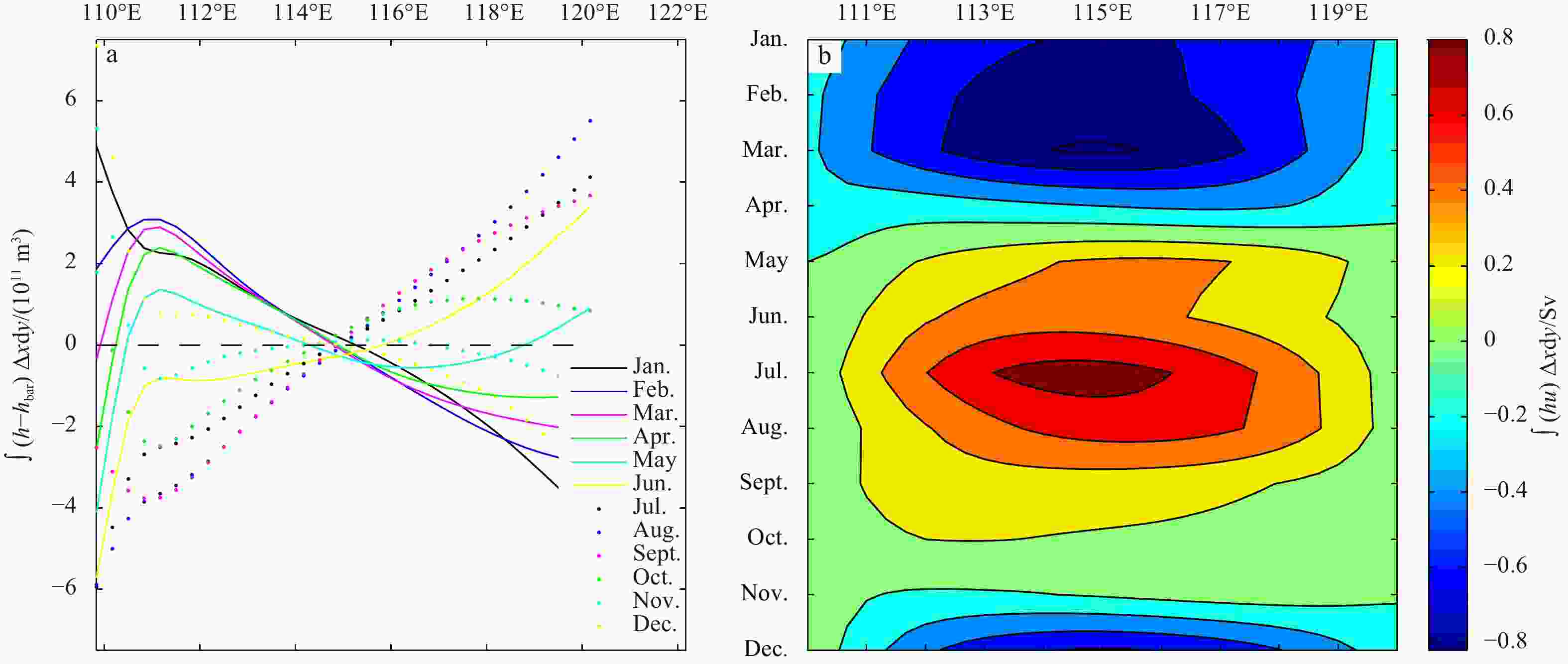
Figure 9. Experiments forced by idealized monthly zonal/meridional wind (Exp. 2). a. Total volumetric anomaly at each longitude band; b. meridionally integrated monthly mean zonal volumetric flux (1 Sv=106 m3/s).
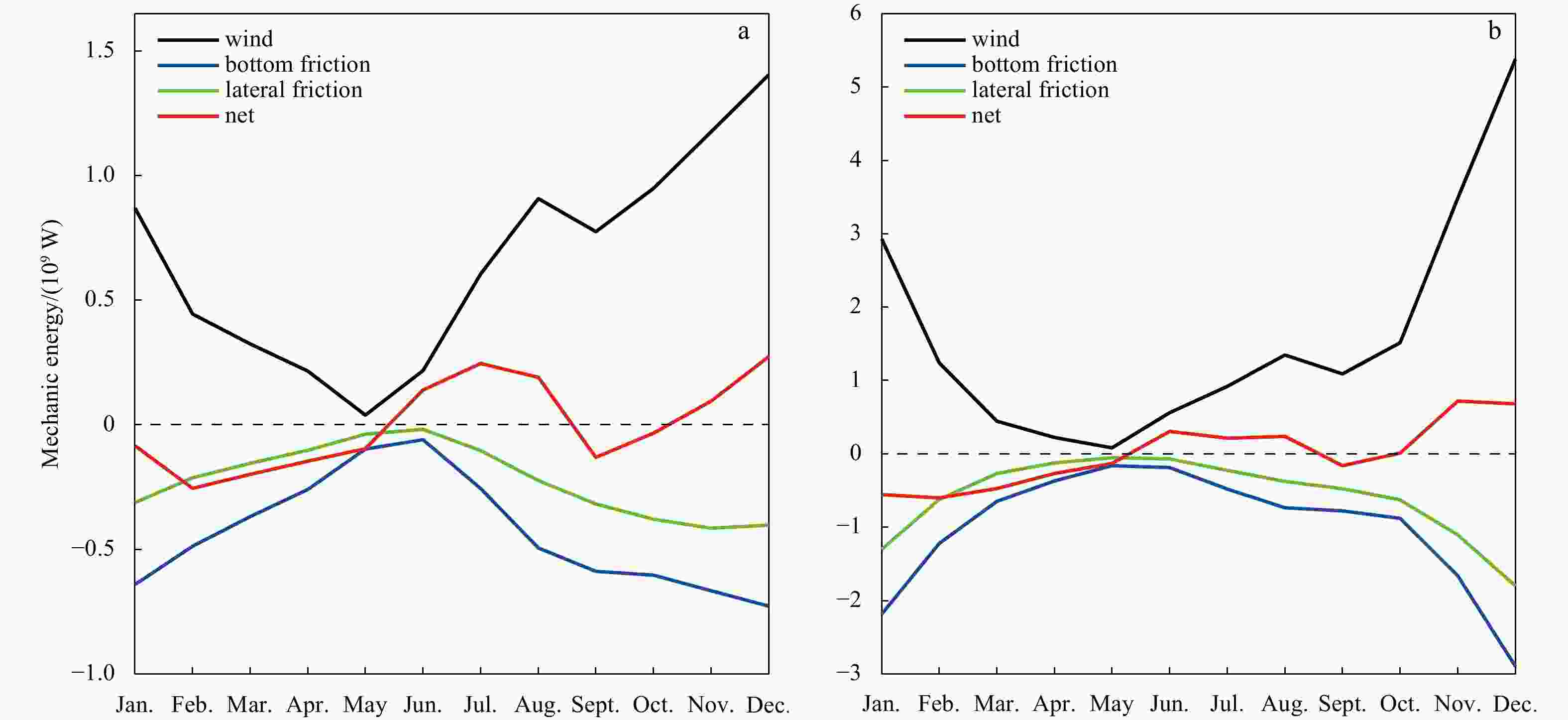
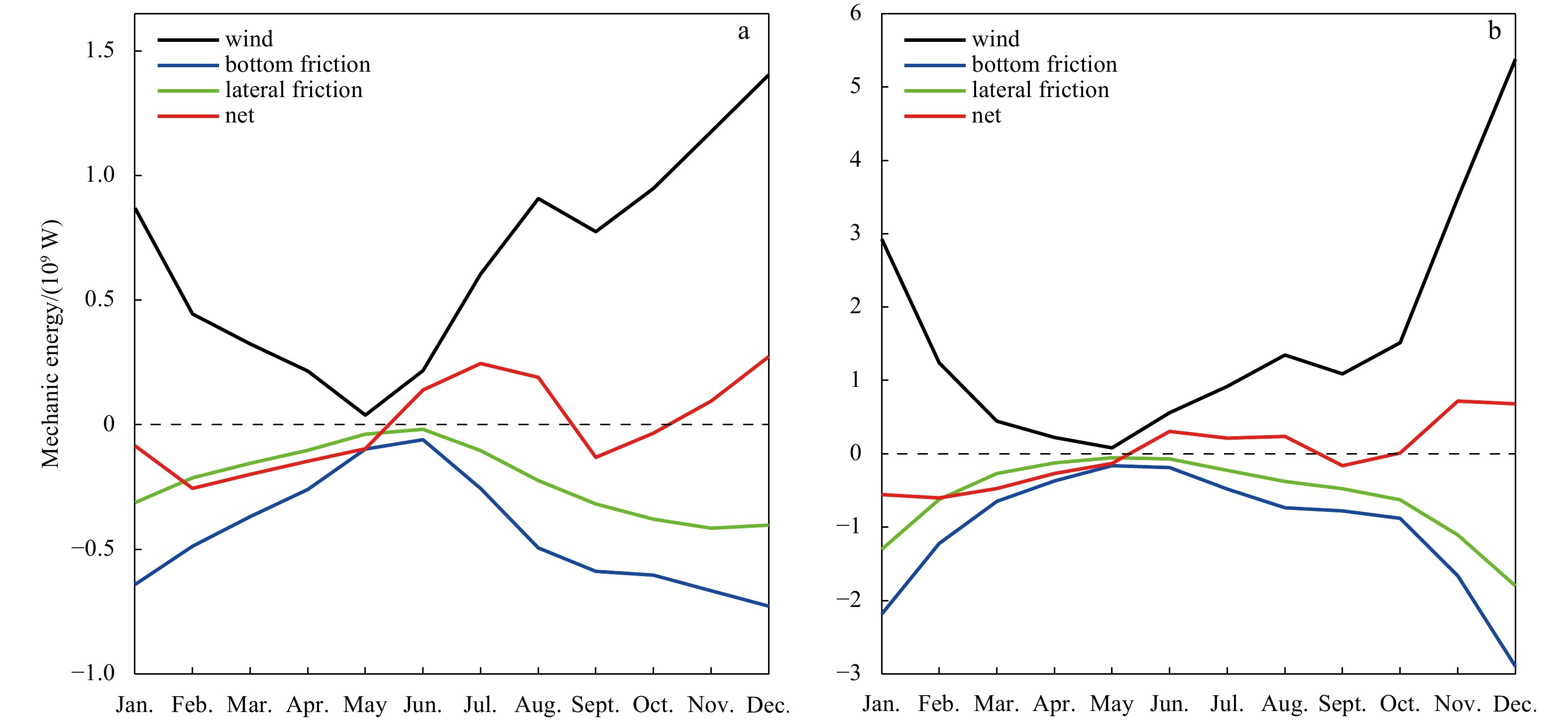
Figure 10. Annual cycle of mechanic energy balance. a. For the model forced by zonal wind stress only (Exp. 1); b. for the model forced by two-dimensional zonal/meridional wind (Exp. 3).
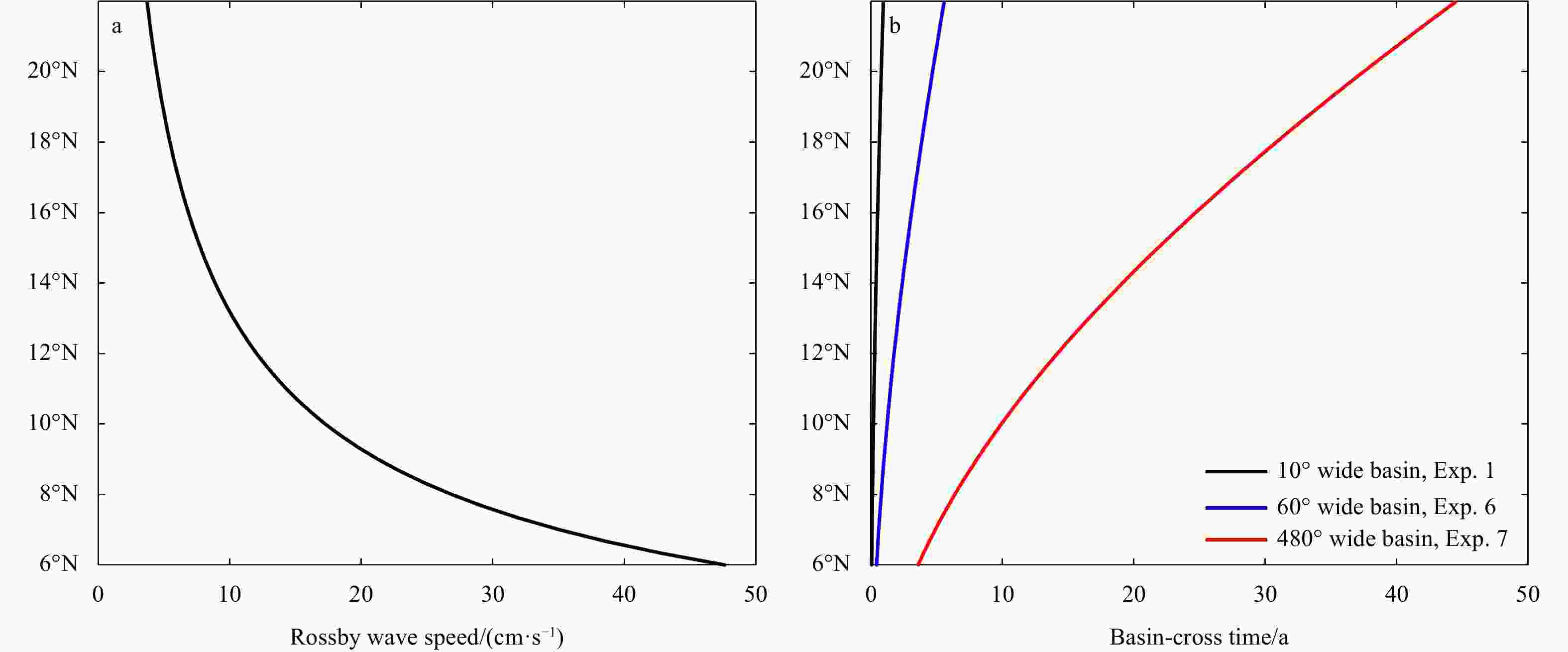
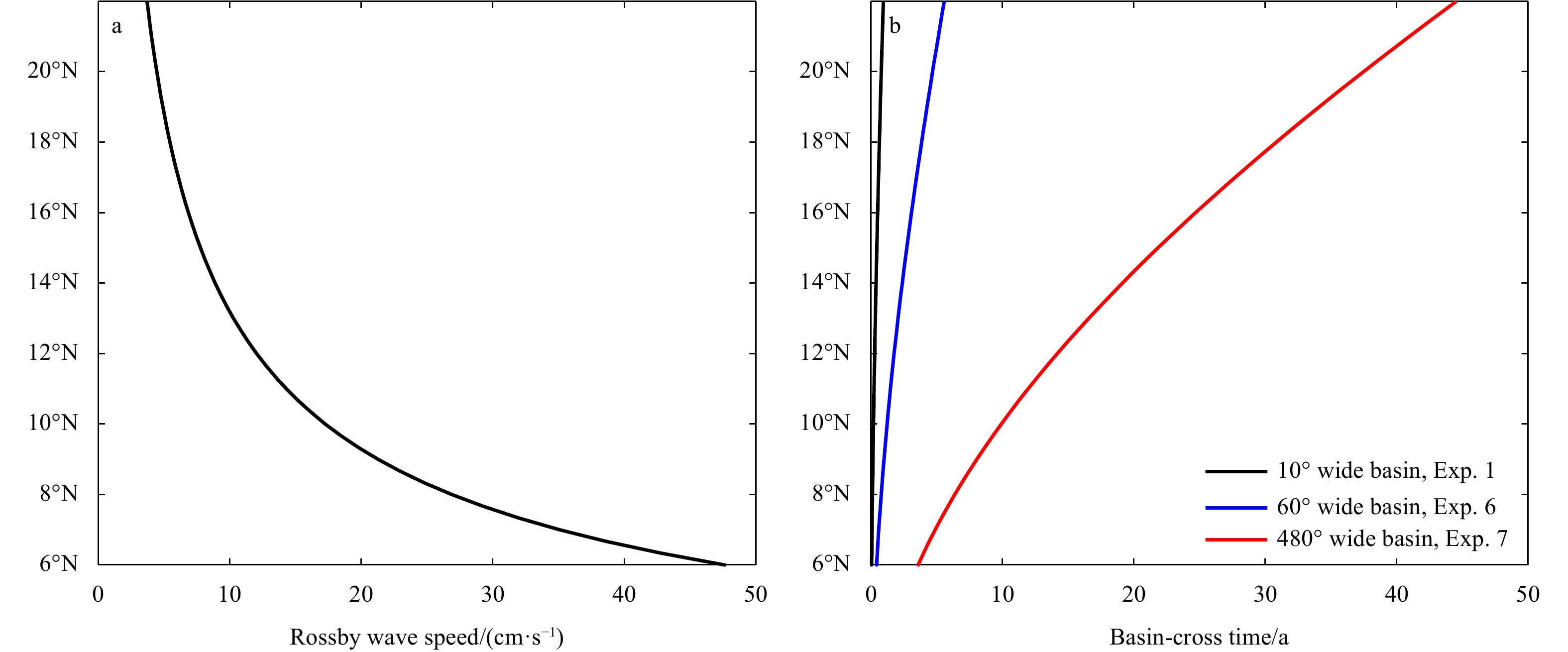
Figure 12. Rossby wave speed (a) and the cross-basin time (b) for the models with the same meridional location, but different zonal width (Exps 1, 6, 7).
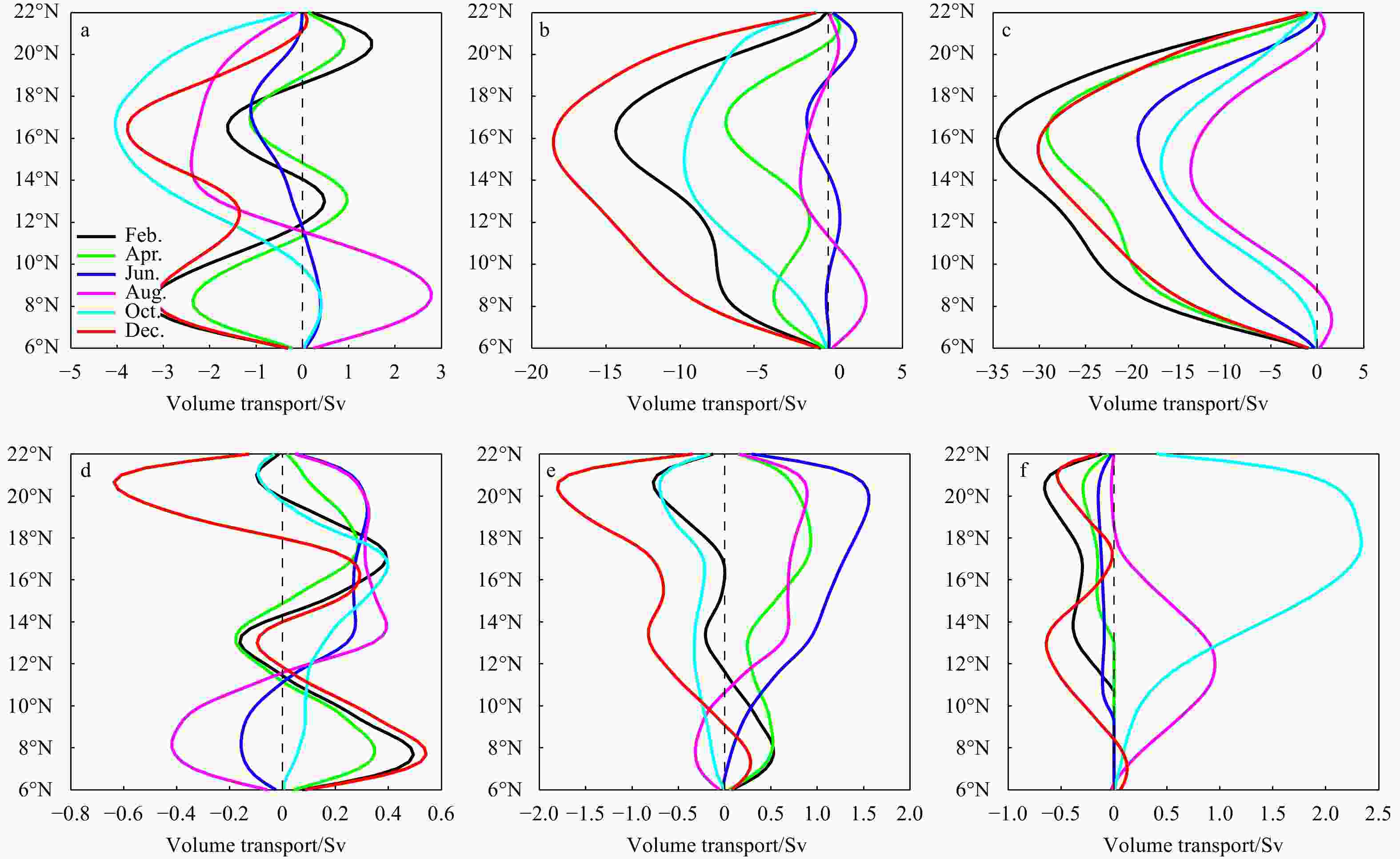
Figure 13. Latitudinal distribution of volume transport based on models with the same meridional range of 6°–22°N, but different zonal width of 10° (Exp. 1, a, d), 60° (Exp. 6, b, e), and 480° (Exp. 7, c, f) for western boundary current (a−c) and eastern boundary current (d−f) (1 Sv=106 m3/s).
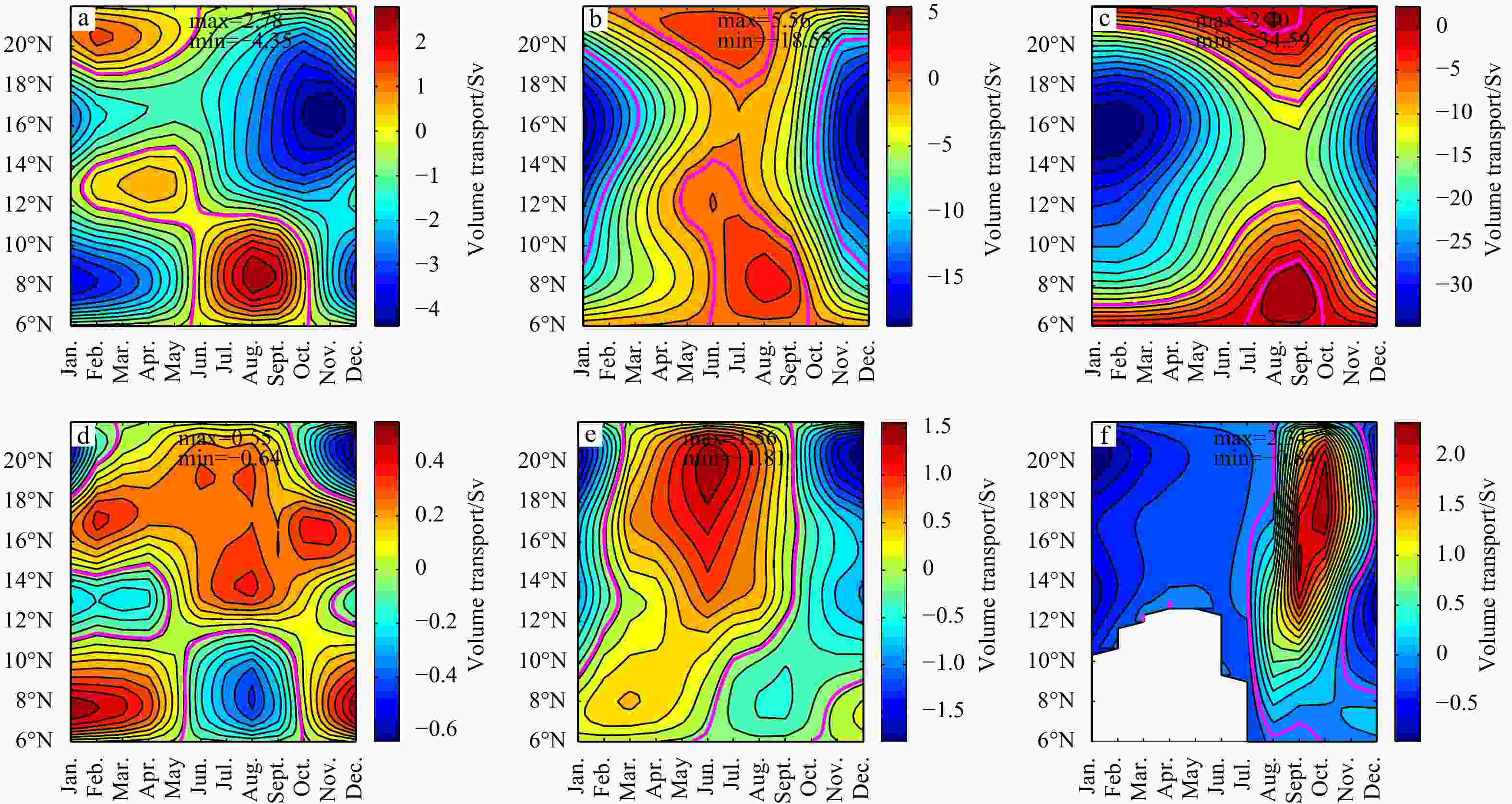
Figure 14. Time-latitude diagram of volumetric transport of the western boundary current (a−c) and eastern boundary current (d−f) for models with the same meridional range of 6°–22°N , but different zonal width of 10° (Exp. 1, a, d), 60° (Exp. 6, b, e), and 480° (Exp. 7, c, f). The magenta curves indicate the zero contours (1 Sv=106 m3/s).
Table 1. Idealized wind stress data used in the model experiments
Zonally mean zonal
wind stressZonally mean zonal wind stress and meridionally
mean meridional wind stressTwo-dimensional wind stress Expression $ {\overline {{\tau ^x}\left( {y,m} \right)} ^x} $ $ {\overline {{\tau ^x}\left( {y,m} \right)} ^x} $,$ {\overline {{\tau ^y}\left( {x,m} \right)} ^y} $ ${ {\tau ^x}\left( {x,y,m} \right),{\tau ^y}\left( {x,y,m} \right)}$ Note: m=(1, …, 12) is the month.  下载: 导出CSV
Table 2. Experiment design
Experiments Meridional range Zonal range Wind stress Run duration/a Exp. 1 6°–22°N 110°–120°E $ {\overline {{\tau ^x}\left( {y,m} \right)} ^x} $ 20 Exp. 2 6°–22°N 110°–120°E $ {\overline {{\tau ^x}\left( {y,m} \right)} ^x} $,$ {\overline {{\tau ^y}\left( {x,m} \right)} ^y} $ 20 Exp. 3 6°–22°N 110°–120°E ${ {\tau ^x}\left( {x,y,m} \right),{\tau ^y}\left( {x,y,m} \right)}$ 20 Exp. 4 0°–16°N 110°–120°E $ {\overline {{\tau ^x}\left( {y,m} \right)} ^x} $ 20 Exp. 5 16°–32°N 110°–120°E $ {\overline {{\tau ^x}\left( {y,m} \right)} ^x} $ 40 Exp. 6 6°–22°N 110°–170°E $ {\overline {{\tau ^x}\left( {y,m} \right)} ^x} $ 60 Exp. 7 6°–22°N 480° $ {\overline {{\tau ^x}\left( {y,m} \right)} ^x} $ 400 Note: Here we expand the width of the model ocean basin to an unrealistic 480°.
下载: 导出CSV
Table 3. Volumetric transport of the western/eastern boundary current (WBC/EBC) for three geographic settings of the model ocean
Western boundary transport Eastern boundary transport Experiment Exp. 1 Exp. 4 Exp. 5 Exp. 1 Exp. 4 Exp. 5 Basin location 6°–22°N 0°–16°N 16°–32°N 6°–22°N 0°–16°N 16°–32°N Maximum/Sv 2.78 2.98 1.69 0.54 0.62 0.55 Minimum/Sv −4.35 −4.22 −4.44 −0.64 −0.57 −0.73
下载: 导出CSV
-
[1] Cai Shuqun, Long Xiaomin, Wu Renhao, et al. 2008. Geographical and monthly variability of the first baroclinic Rossby radius of deformation in the South China Sea. Journal of Marine Systems, 74(1–2): 711–720. doi: 10.1016/j.jmarsys.2007.12.008 [2] Chu P C, Edmons N L, Fan Chenwu. 1999. Dynamical mechanisms for the South China Sea seasonal circulation and thermohaline variabilities. Journal of Physical Oceanography, 29(11): 2971–2989. doi: 10.1175/1520-0485(1999)029<2971:DMFTSC>2.0.CO;2 [3] Fang Wendong, Fang Guohong, Shi Ping, et al. 2002. Seasonal structures of upper layer circulation in the southern South China Sea from in situ observations. Journal of Geophysical Research: Oceans, 107(C11): 3202. doi: 10.1029/2002JC001343 [4] Gan Jianping, Li H, Curchitser E N, et al. 2006. Modeling South China Sea circulation: Response to seasonal forcing regimes. Journal of Geophysical Research: Oceans, 111(C6): C06034 [5] He Zhigang, Lyu Kewei, Quan Qi. 2020. The South China Sea western boundary current. In: Hu J, Ho C R, Xie L, et al., eds. Regional Oceanography of the South China Sea. Singapore: World Scientific, 77–99 [6] Huang Rui xin. 1986. Numerical simulation of wind-driven circulation in a subtropical/subpolar basin. Journal of Physical Oceanography, 16(10): 1636–1650. doi: 10.1175/1520-0485(1986)016<1636:NSOWDC>2.0.CO;2 [7] Huang Rui xin. 2010. Ocean Circulation: Wind-Driven and Thermohaline Processes. Cambridge: Cambridge University Press [8] Liang Xiangshan. 2017. The seasonally varying monsoon wind may suppress the western boundary current in the South China Sea. Oceanography & Fisheries Open Access Journal, 3(1): 555601 [9] Pedlosky J. 1965. A study of the time dependent ocean circulation. Journal of the Atmospheric Sciences, 22(3): 267–272. doi: 10.1175/1520-0469(1965)022<0267:ASOTTD>2.0.CO;2 [10] Qu Tangdong. 2000. Upper-layer circulation in the South China Sea. Journal of Physical Oceanography, 30(6): 1450–1460. doi: 10.1175/1520-0485(2000)030<1450:ULCITS>2.0.CO;2 [11] Shaw P T, Chao S Y, Fu L L. 1999. Sea surface height variations in the South China Sea from satellite altimetry. Oceanologica Acta, 22(1): 1–17. doi: 10.1016/S0399-1784(99)80028-0 [12] Stommel H. 1948. The westward intensification of wind-driven ocean currents. Eos, Transactions American Geophysical Union, 29(2): 202–206 [13] Wang Guihua, Chen Dake, Su Jilan. 2006. Generation and life cycle of the dipole in the South China Sea summer circulation. Journal of Geophysical Research: Oceans, 111: C06002 [14] Wyrtki K. 1961. Physical oceanography of the Southeast Asian waters. La Jolla: The University of California [15] Yang Haijun, Liu Qinyu. 2003. Forced Rossby wave in the northern South China Sea. Deep-Sea Research Part I: Oceanographic Research Papers, 50(7): 917–926. doi: 10.1016/S0967-0637(03)00074-8 [16] Yang Haijun, Liu Qinyu, Liu Zhengyu, et al. 2002. A general circulation model study of the dynamics of the upper ocean circulation of the South China Sea. Journal of Geophysical Research: Oceans, 107(C7): 22-1–22-14 [17] Yang Jiayan, Price James F. 2000. Water-mass formation and potential vorticity balance in an abyssal ocean circulation. Journal of Marine Research, 58: 789−808. -


 点击查看大图
计量
- 文章访问数: 399
- HTML全文浏览量: 119
- PDF下载量: 25
- 被引次数: 0