

Variations of suspended sediment transport caused by changes in shoreline and bathymetry in the Zhujiang (Pearl) River Estuary in the wet season
-
Abstract: A wave-current-sediment coupled numerical model is employed to study the responses of suspended sediment transport in the wet season to changes in shoreline and bathymetry in the Zhujiang (Pearl) River Estuary (ZRE) from 1971 to 2012. It is shown that, during the wavy period, the large wave-induced bottom stress enhances sediment resuspension, resulting in an increase in the area of suspended sediment concentration (SSC) greater than 100 mg/L by 183.4%. On one hand, in spring tide, the change in shoreline reduces the area of SSC greater than 100 mg/L by 17.8% in the west shoal (WS) but increases the SSC, owing to the closer sediment source to the offshore and the stronger residual current at the Hengmeng (HEM) and Hongqili (HQL) outlets. The eastward Eulerian transport is enhanced in the WS and west channel (WC), resulting in a higher SSC there. The reclamation of Longxue Island (LXI) increases SSC on its east side and east shoal (ES) but decreases the SSC on its west and south sides. Moreover, in the WC, the estuarine turbidity maximum (ETM) is located near the saltwater wedge and moves southward, which is caused by the southward movement of the maximum longitudinal Eulerian transport. In neap tide, the changes are similar but relatively weaker. On the other hand, in spring tide, the change in bathymetry makes the SSC in the WS increase, and the area of SSC greater than 100 mg/L increases by 11.4% and expands eastward and southward, which is caused by the increases in wave-induced bottom stress and eastward Eulerian transport. On the east side of the WC, the eastward Eulerian transport decreases significantly, resulting in a smaller SSC in the middle shoal (MS). In addition, in the WC, the maximum SSC is reduced, which is caused by the smaller wave-induced bottom stress and a significant increase of 109.88% in southward Eulerian transport. The results in neap tide are similar to those in spring tide but with smaller changes, and the sediment transports northward in the WC owing to the northward Eulerian transport and vertical shear transport. This study may provide some references for marine ecological environment security and coastal management in the ZRE and other estuaries worldwide affected by strong human interventions.
-
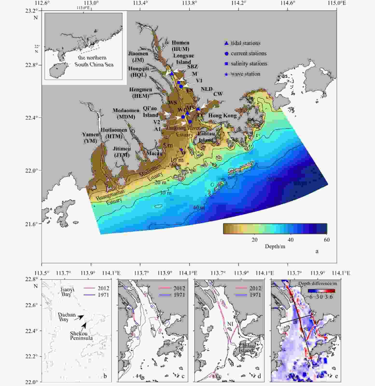
Figure 1. Model domain, shorelines and water depth modified from Lin et al. (2021). a. Model domain (zoomed-in dashed line rectangle box in the top left corner) and bathymetry in the ZRE (shoreline and water depth are drawn from the nautical charts of 2012). WS, WC, MS, EC, and ES represent the west shoal, west channel, middle shoal, east channel and east shoal, respectively. NI represents Neilingding Island. SBZ, CW, and NLD represent Shanbanzhou, Chiwan, and Neilingding, respectively, which are tidal stations. V1 and V2 are current stations, A1 and M are salinity stations, and W is a wave station. b. Shorelines, c. 5 m isobaths and d. 10 m isobaths in the ZRE, in which the red and blue lines represent the 2012 and 1971 cases, respectively. e. Water depth difference between 2012 and 1971. Sections A and B in e are used in the following analysis.
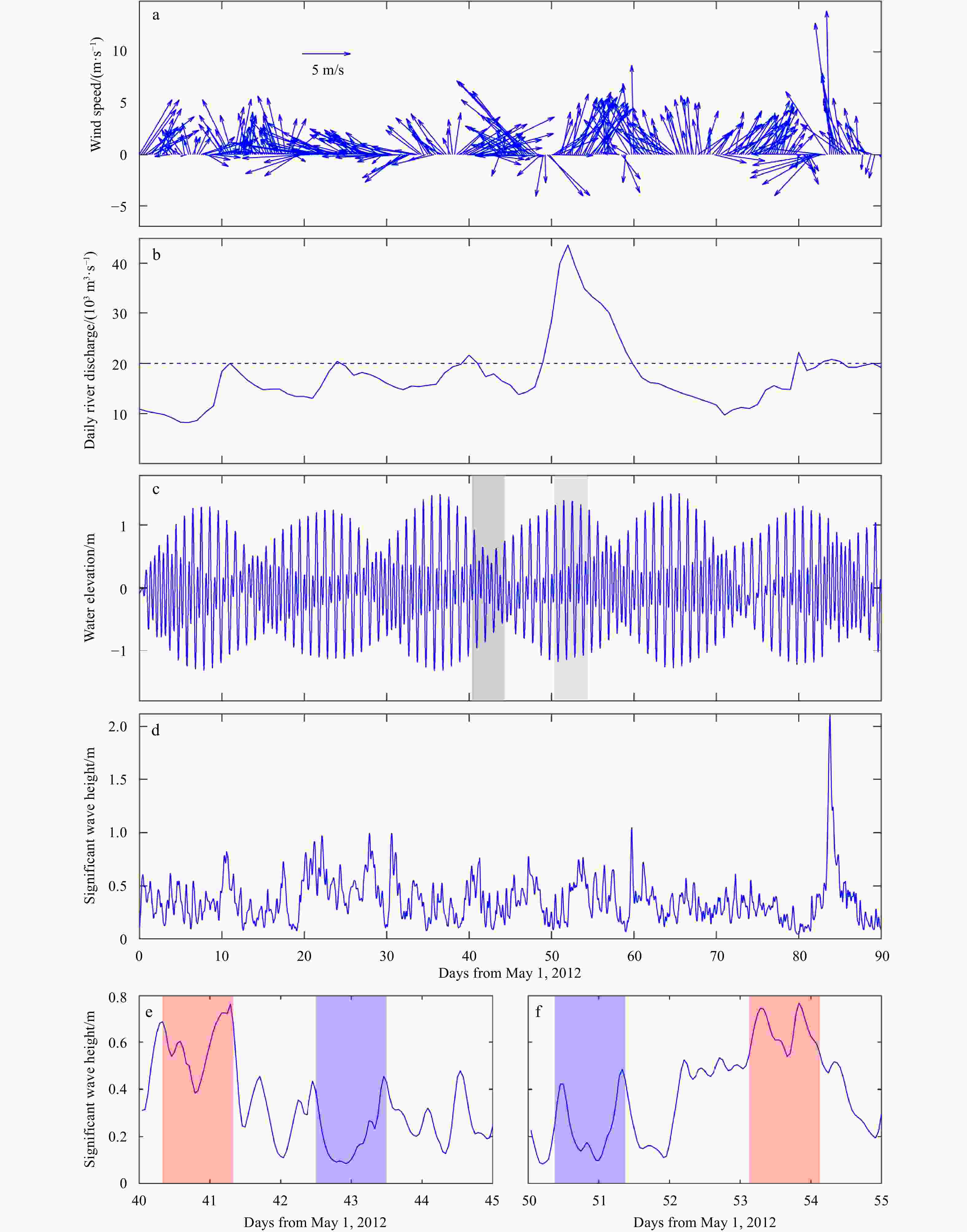
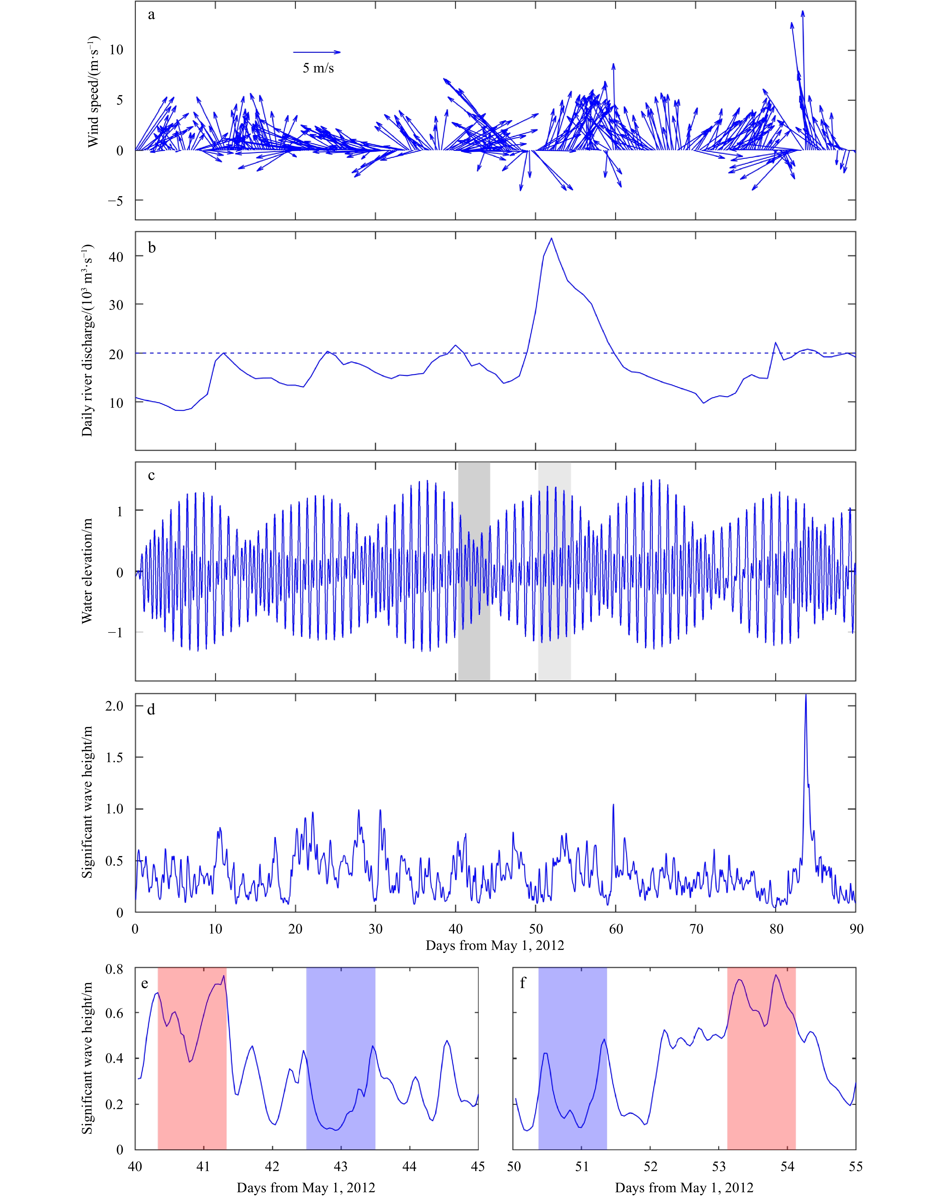
Figure 2. Time series of wind speed at NLD (a), daily river discharge rate in the ZRE (b), water elevation at NLD (c), and significant wave height at NLD (d) from May 1, 2012, and the significant wave heights in neap (e) and spring (f) periods derived from d. The dark and light gray shadows in c are chosen as neap tide and spring tide periods, respectively, in this paper. The red and blue shadows in e and f are chosen as wavy and calm periods, respectively.

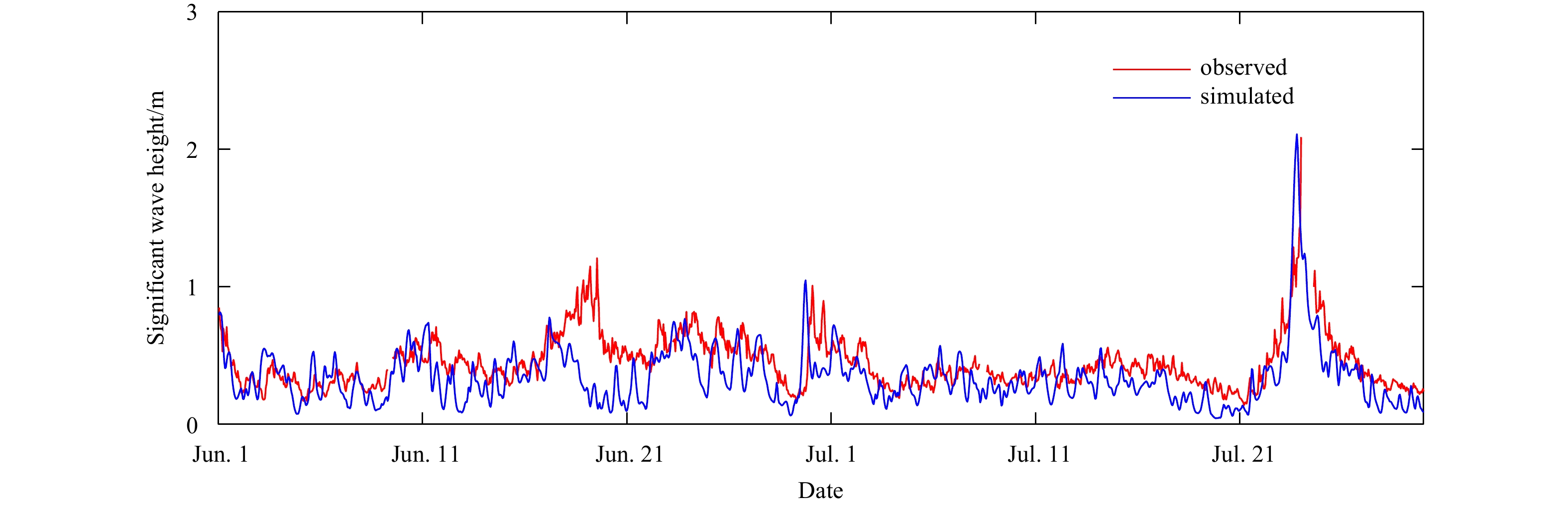
Figure 3. Observed and simulated significant wave heights at Sta. W. The red and blue lines represent the observed and simulated results, respectively.
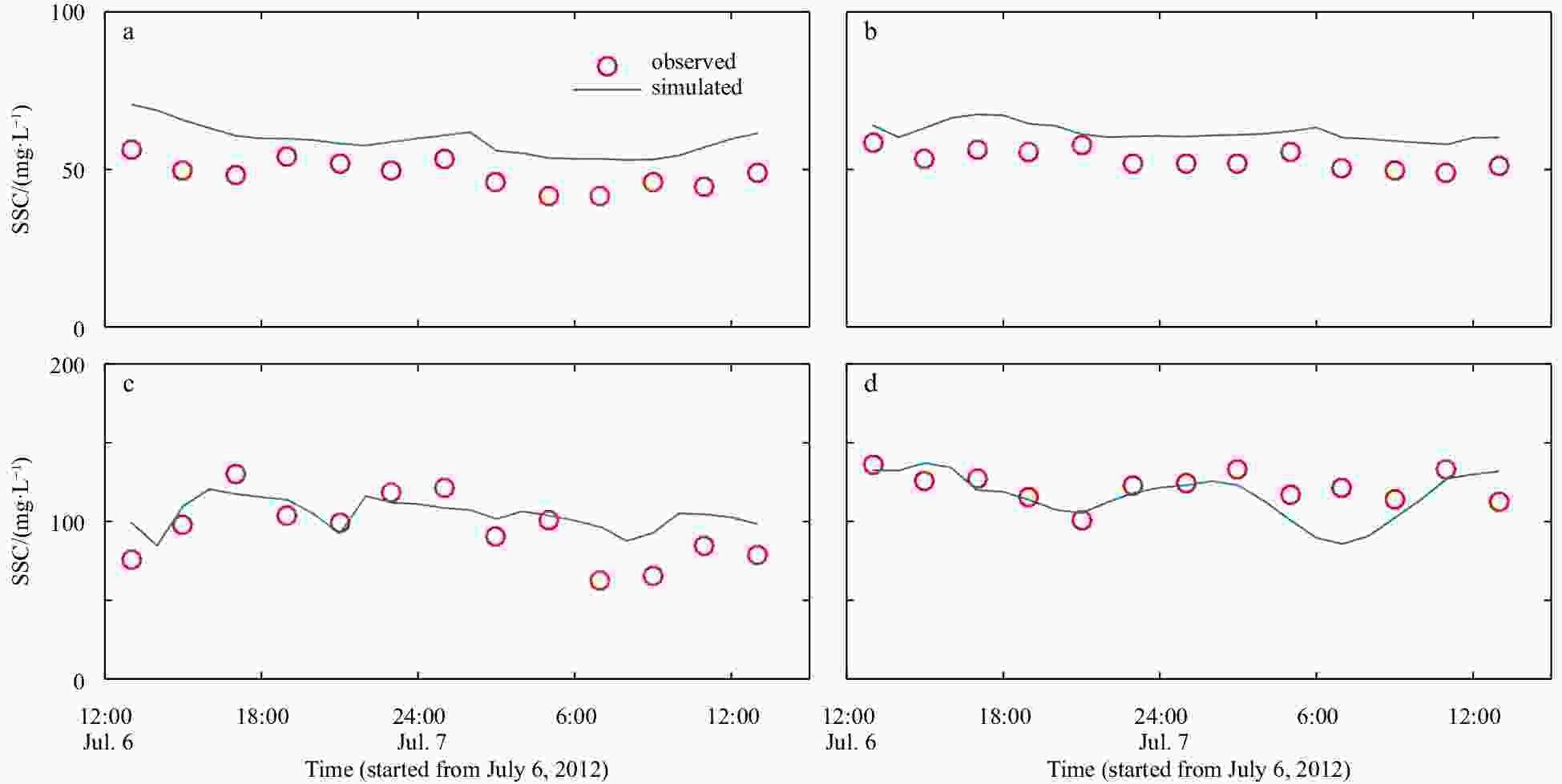
Figure 4. Observed and simulated SSC at Sta. V1 surface (a) and bottom (b) and at Sta. V2 surface (c) and bottom (d). The red hollow circles and the blue lines represent the observed and simulated results, respectively.
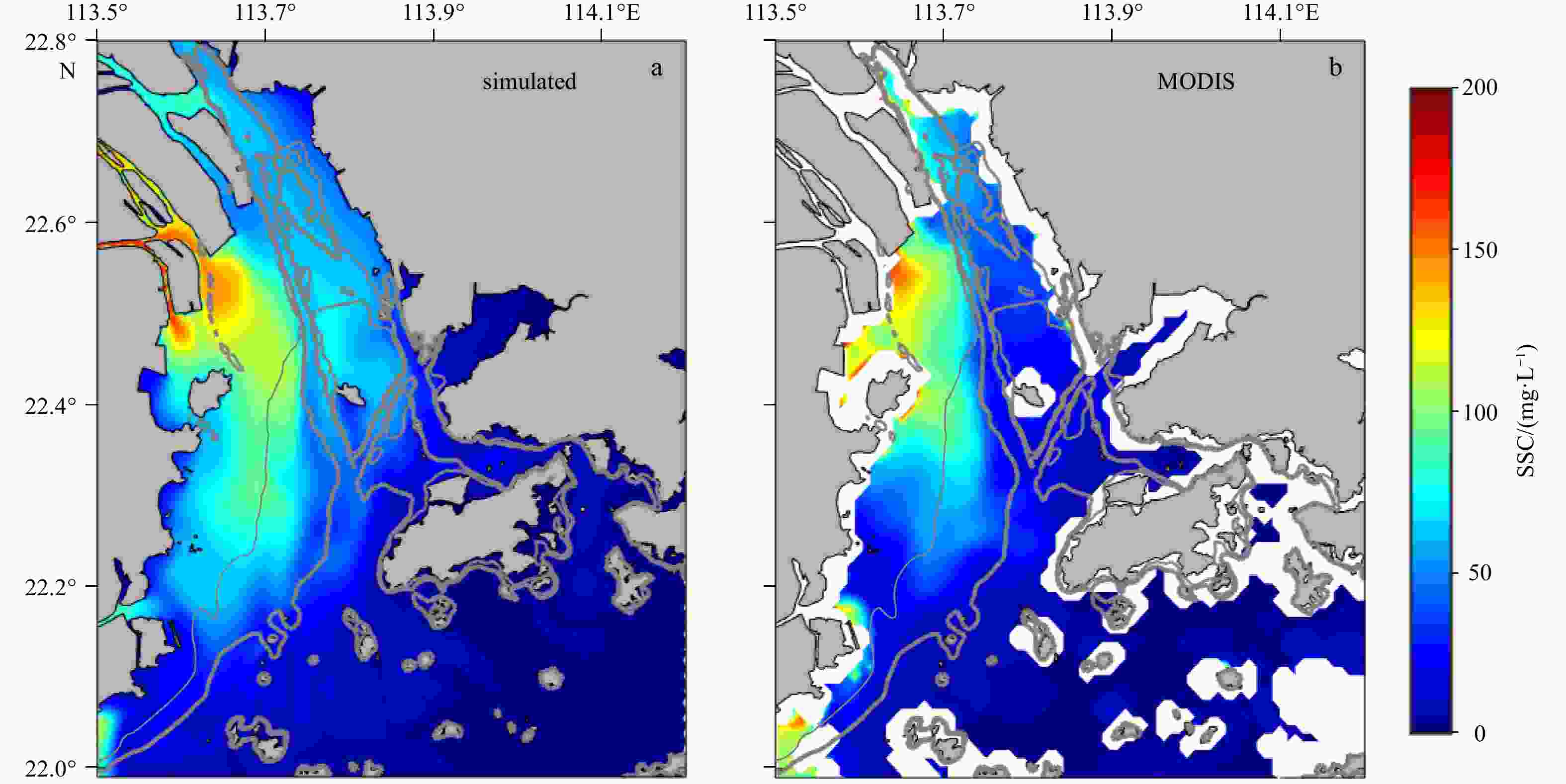
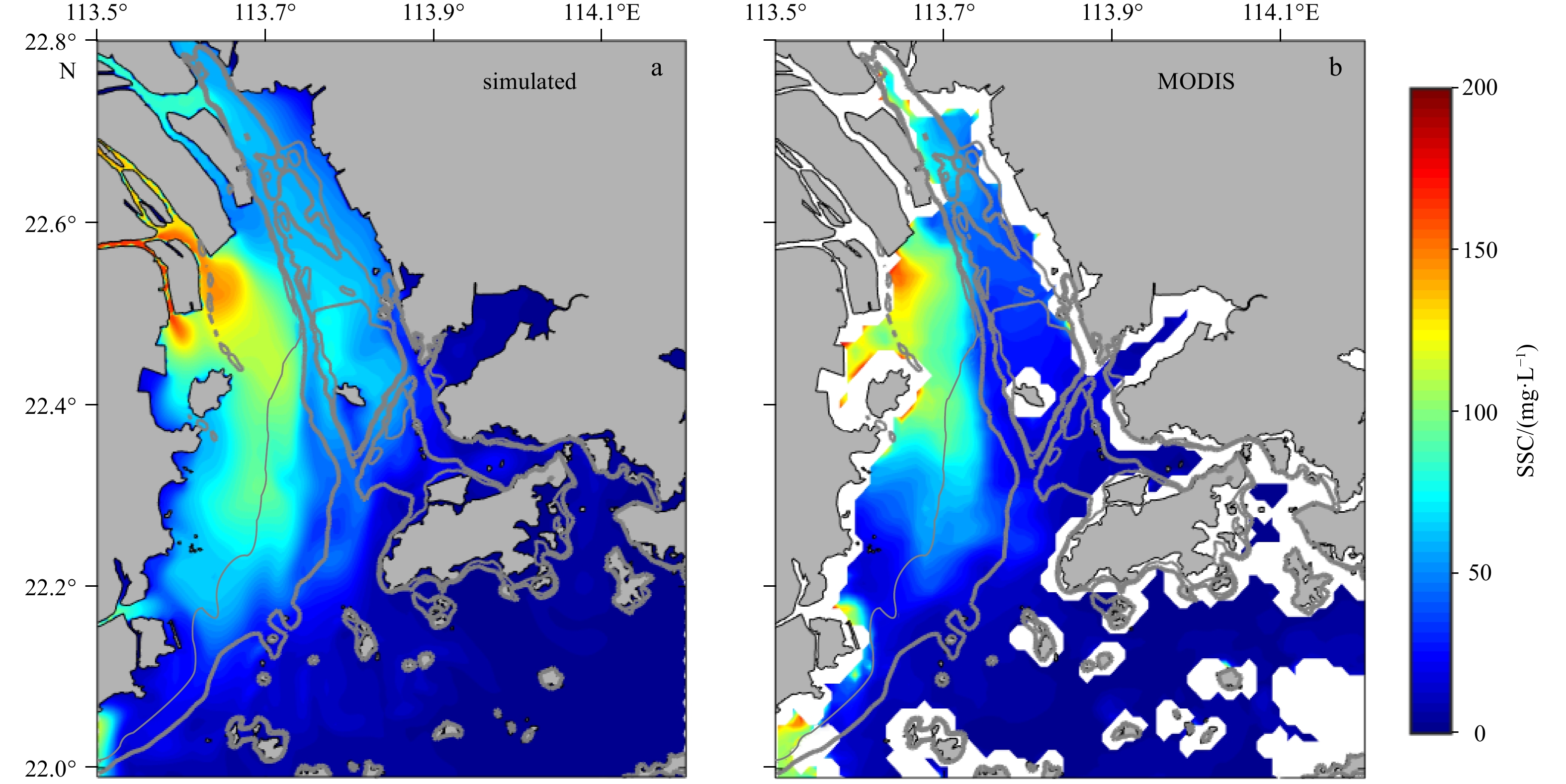
Figure 5. Surface SSC distributions obtained from the model results (a) and moderate resolution imaging spectroradiometer (MODIS) data (b) on June 28, 2012. Thin/thick gray lines denote 6 m/8 m isobaths.
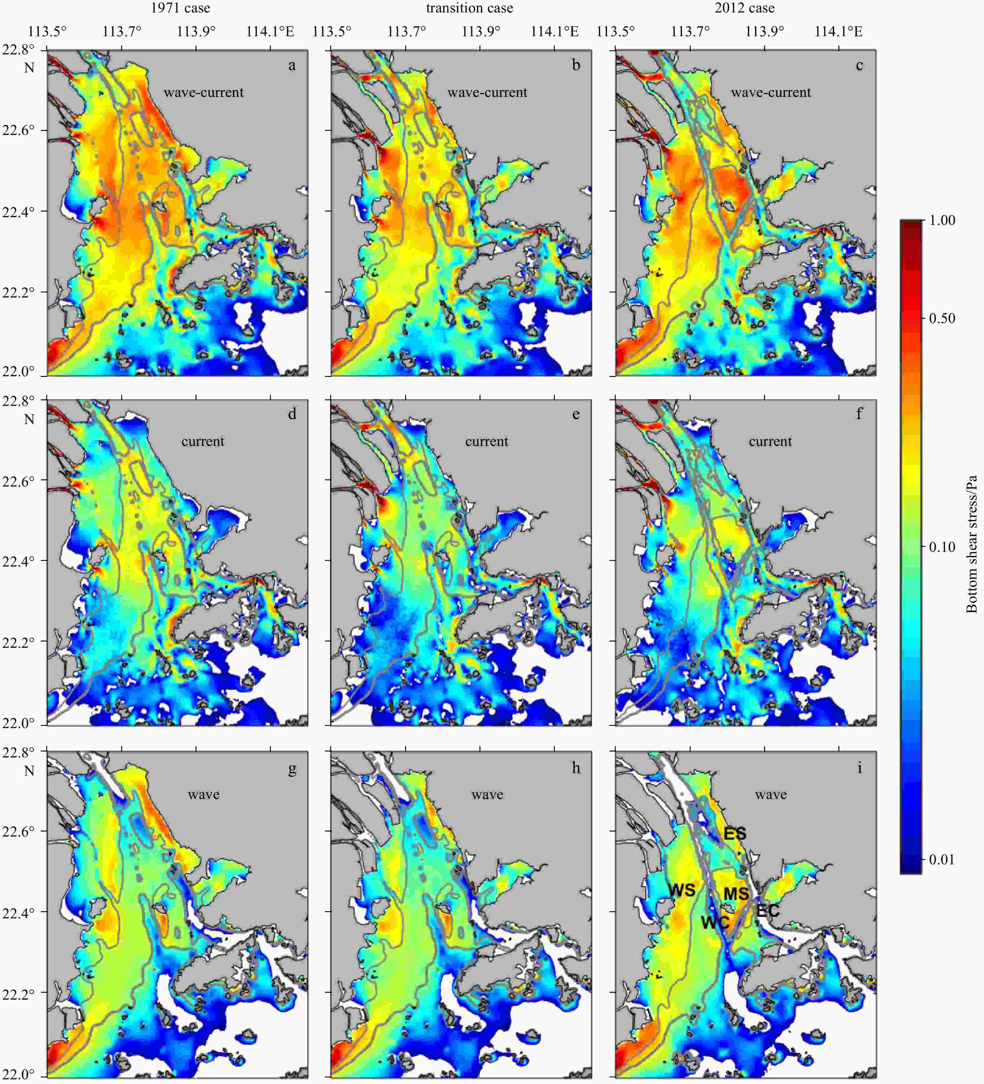
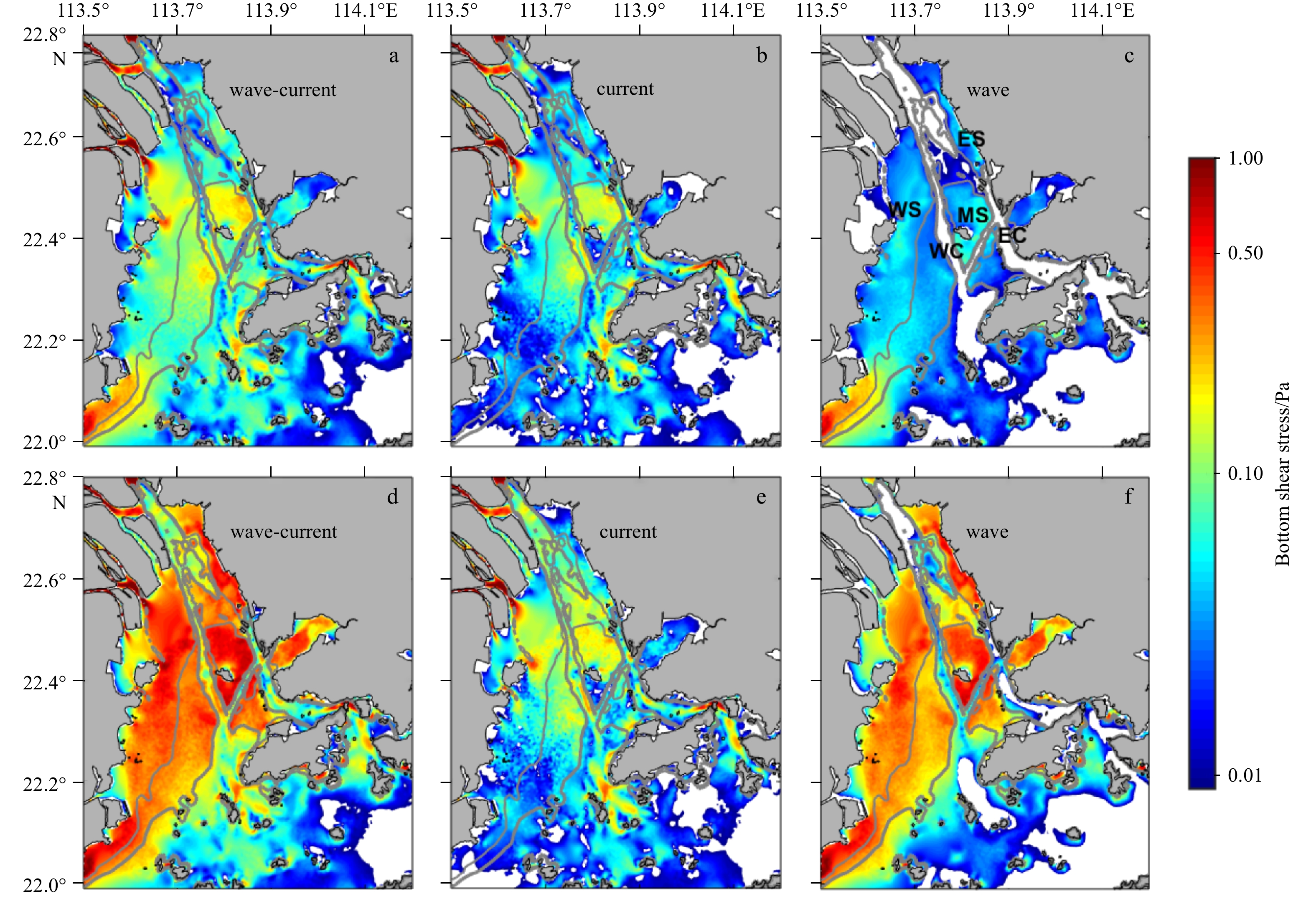
Figure 6. Tidal averaged bottom shear stress in spring tide. a–c. Wave-current combined, d–f. current-induced, and g–i. wave-induced. Note that the bottom shear stress is on a log scale. The white areas correspond to bottom stress below 0.01 Pa. Thin/thick gray lines indicate 6 m/8 m isobaths. The 1971, transition and 2012 cases are indicated in the left, middle and right panels, respectively.
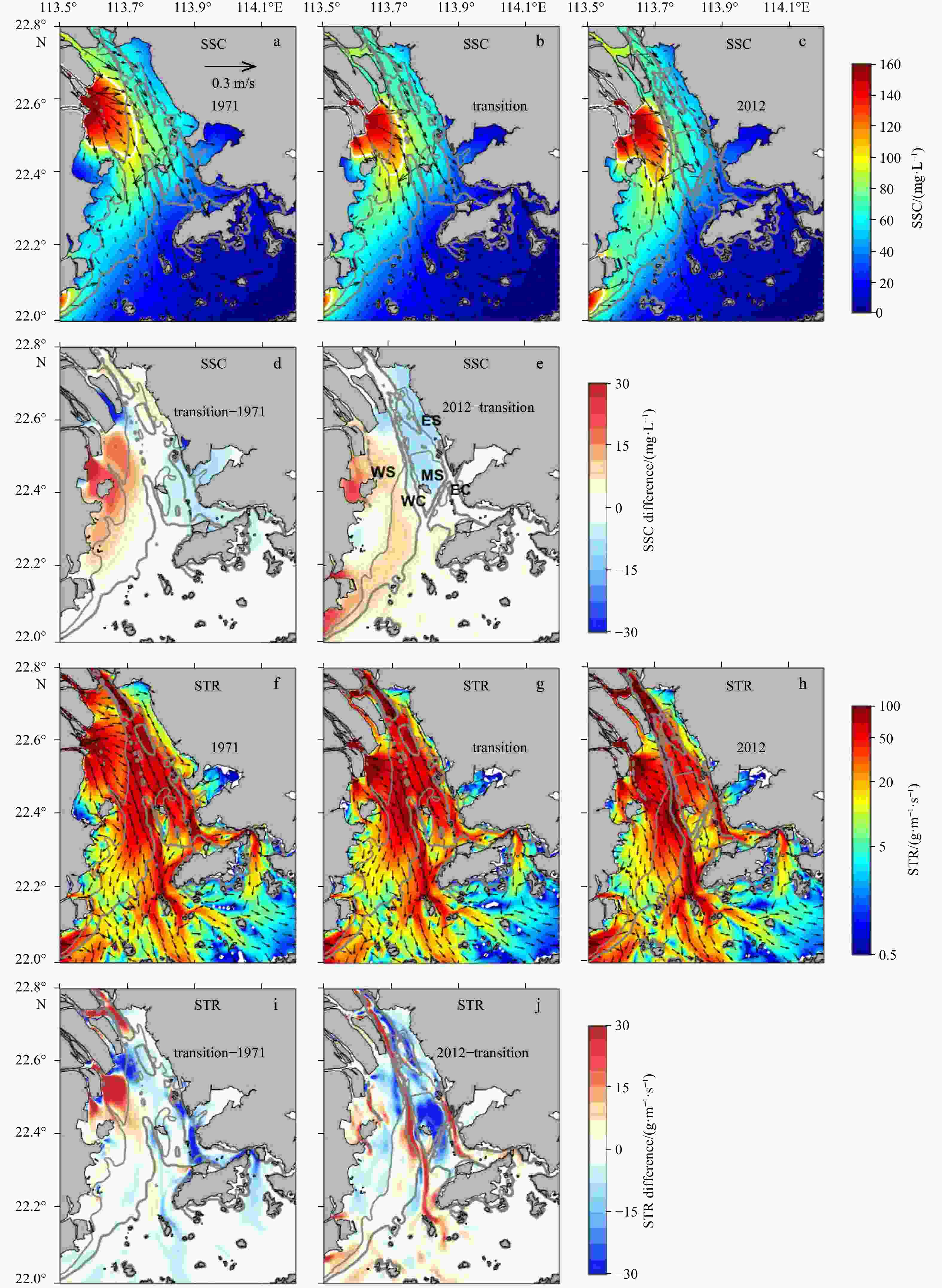
Figure 7. Distributions of tidally and vertically averaged SSC (contour) and residual current (arrow), and tidally averaged and depth-integrated bottom shear stress in spring tide: a and f. 1971 case, b and g. transition case, c and h. 2012 case, d and i. the difference calculated by the transition case–1971 case, and e and j. the difference calculated by 2012 case–transition case. The arrows in f–h indicate the direction of bottom shear stress, and white areas indicate STR below 0.5 g/(m·s). Thin/thick gray lines denote 6 m/8 m isobaths.
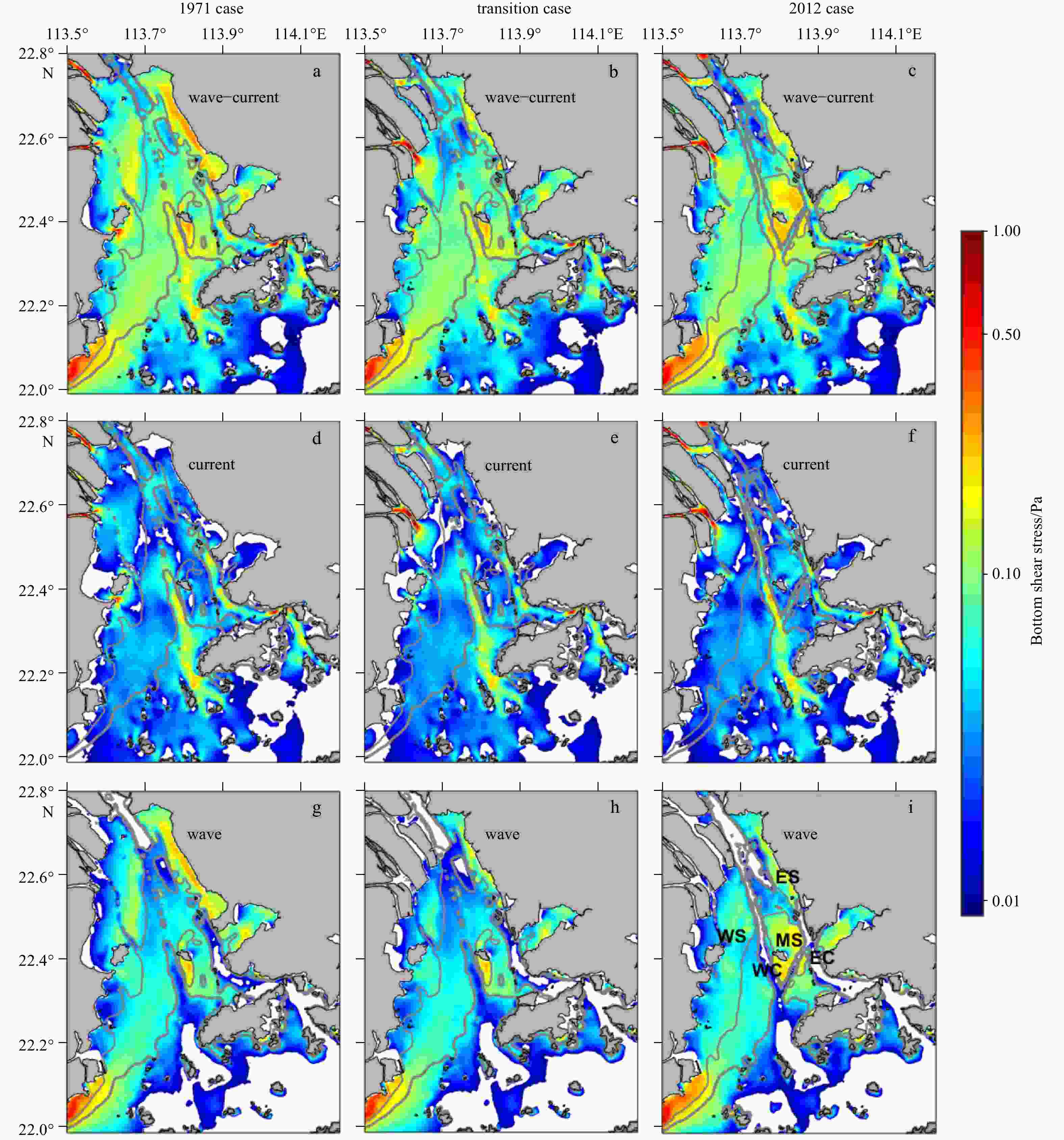
Figure 8. Tidal averaged bottom shear stress in neap tide. a–c. Wave-current combined, d–f. current-induced, and g–i. wave-induced. Note that the bottom shear stress is on a log scale. The white areas correspond to bottom stress below 0.01 Pa. Thin/thick gray lines indicate 6 m/8 m isobaths. The 1971, transition and 2012 cases are indicated in the left, middle and right panels, respectively.
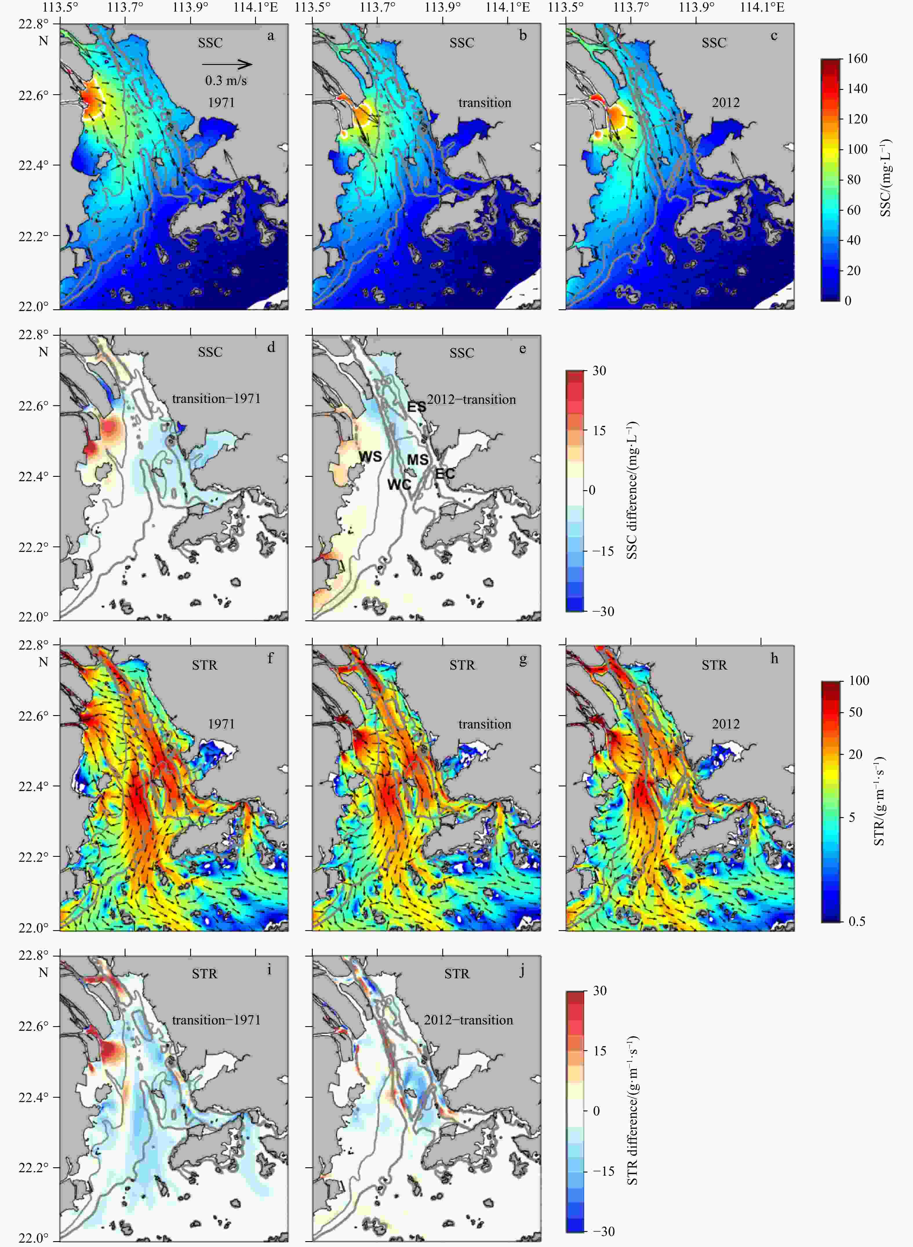
Figure 9. Distributions of tidally and vertically averaged SSC (contour) and residual current (arrow), and tidally averaged and depth-integrated STR in neap tide: a and f. 1971 case, b and g. transition case, c and h. 2012 case, d and i. the difference calculated by the transition case–1971 case, and e and j. the difference calculated by 2012 case–transition case. The arrows in f–h indicate the direction of STR, and white areas indicate STR below 0.5 g/(m·s). Thin/thick gray lines denote 6 m/8 m isobaths.

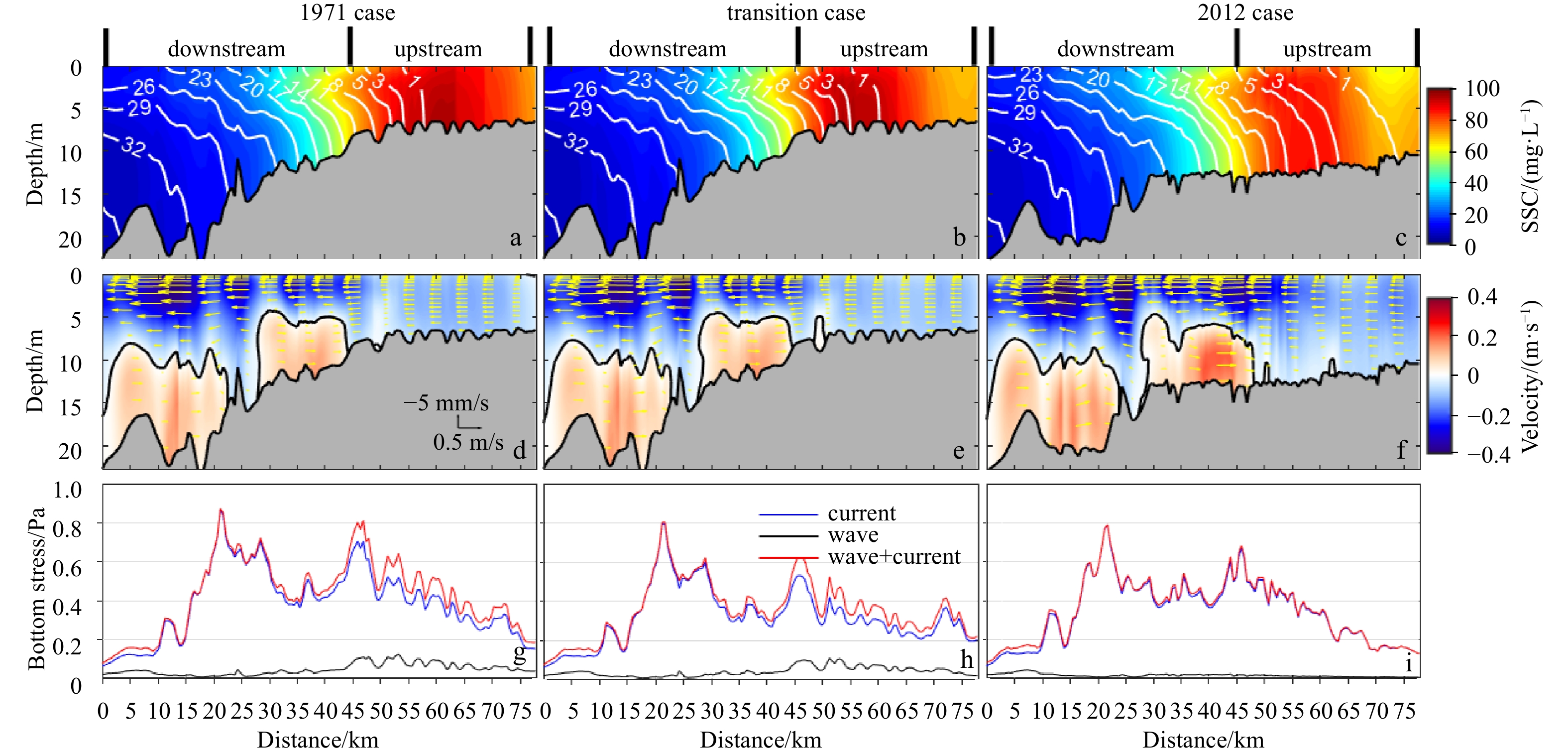
Figure 10. Along-channel distributions of tidally averaged SSC (contours) and salinity (white lines) (a, b, c), along-channel residual current (contours and arrows) (d, e, f), and bed shear (g, h, i) at Section A (shown in Fig. 1e) in spring tide. The positive value for the along-channel residual current is landward, and the zero along-channel residual current is marked by a black solid line. The current-induced, wave-induced and wave-current combined bottom shear stresses are denoted by blue, dark, and red lines, respectively. The 1971, transition and 2012 cases are indicated in the left, middle and right panels, respectively.
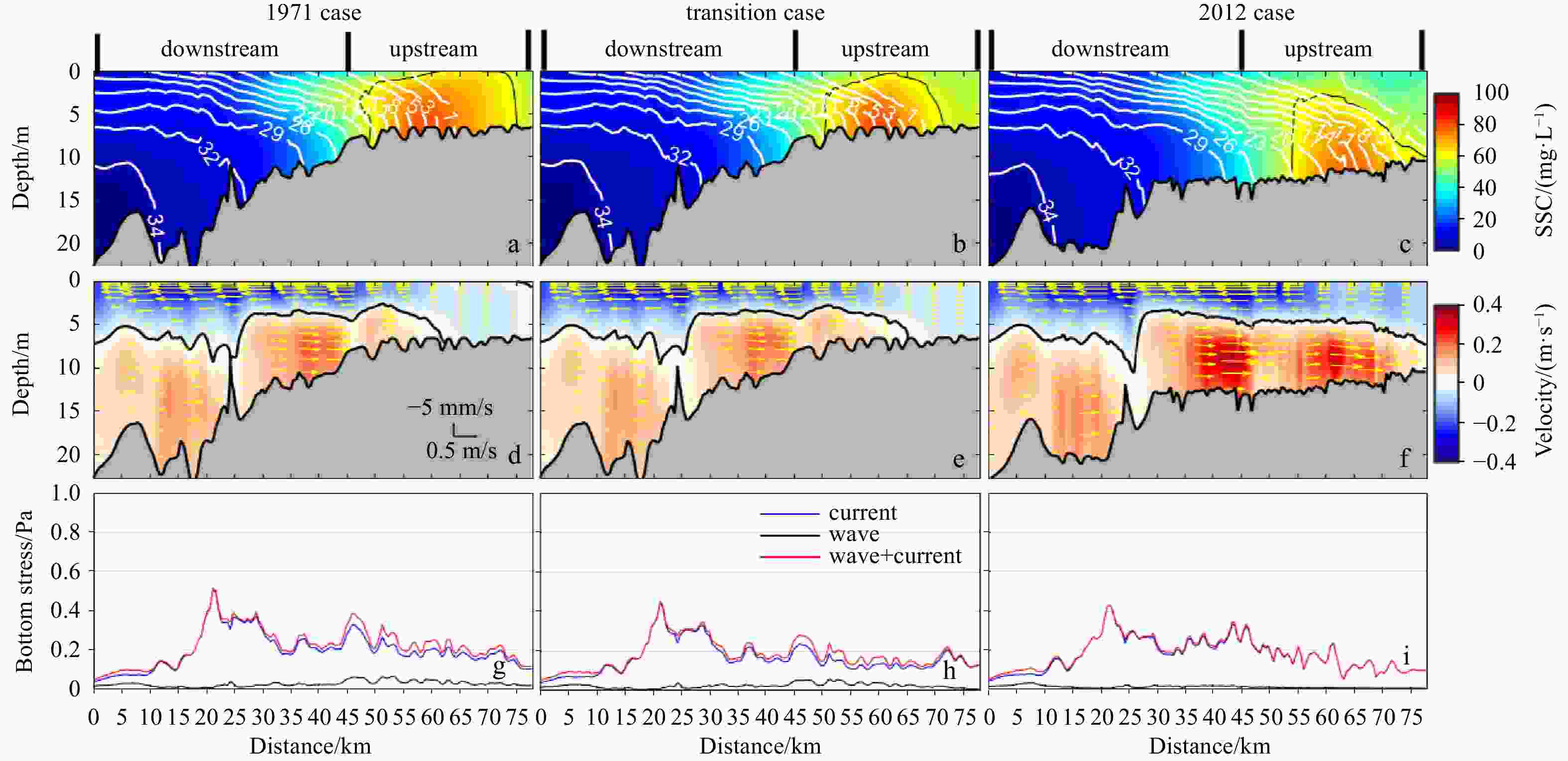
Figure 11. Along-channel distributions of tidally averaged SSC (contours) and salinity (white lines) (a, b, c), along-channel residual current (contours and arrows) (d, e, f), and bed shear (g, h, i) at Section A (shown in Fig. 1e) in neap tide. The positive value for the along-channel residual current is landward, and the zero along-channel residual current is marked by a black solid line. The current-induced, wave-induced and wave-current combined bottom shear stresses are denoted by blue, dark, and red lines, respectively. The SSC of 60 mg/L is marked by a black solid line in a, b and c. The 1971, transition and 2012 cases are indicated in the left, middle and right panels, respectively.
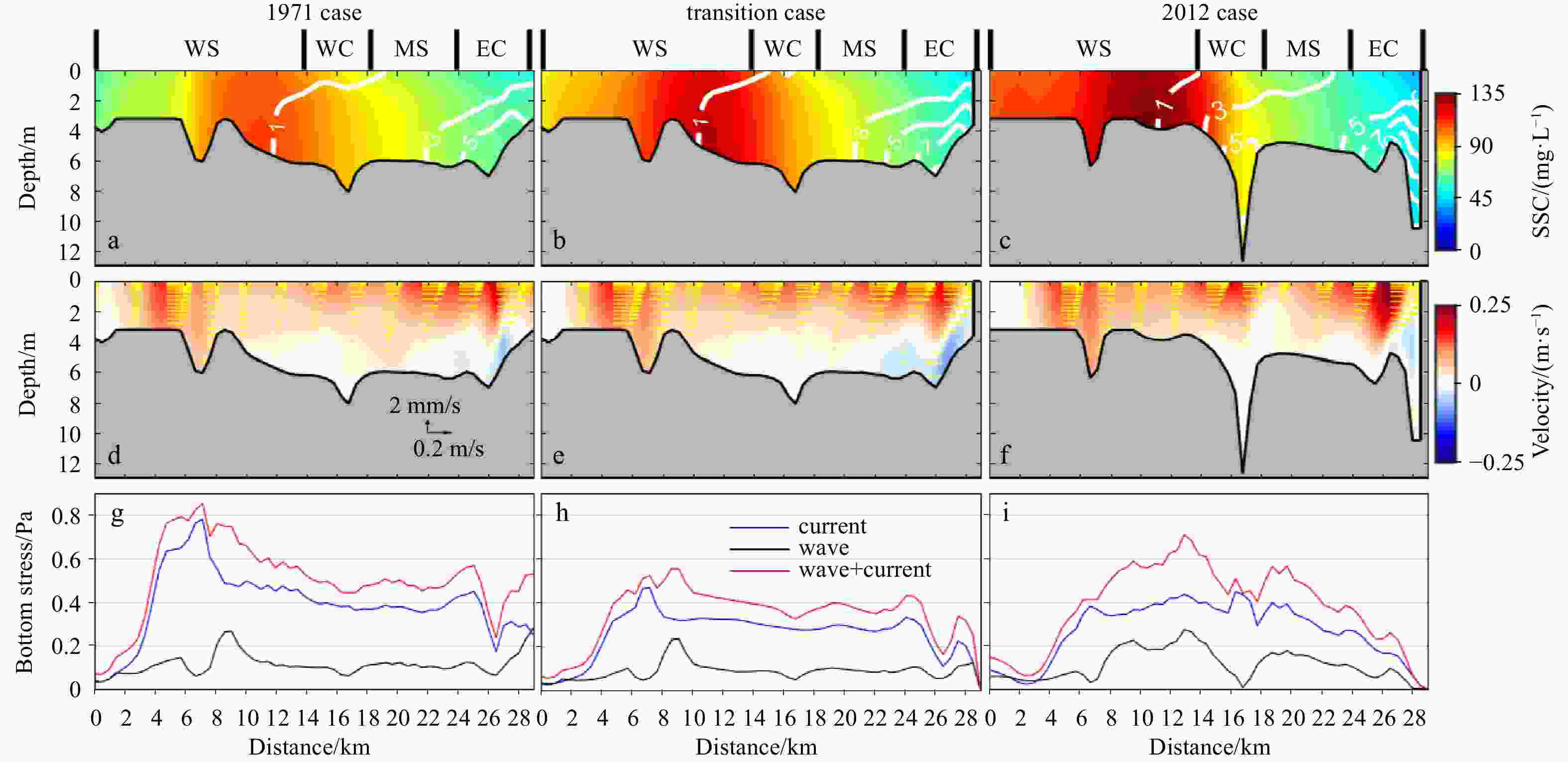
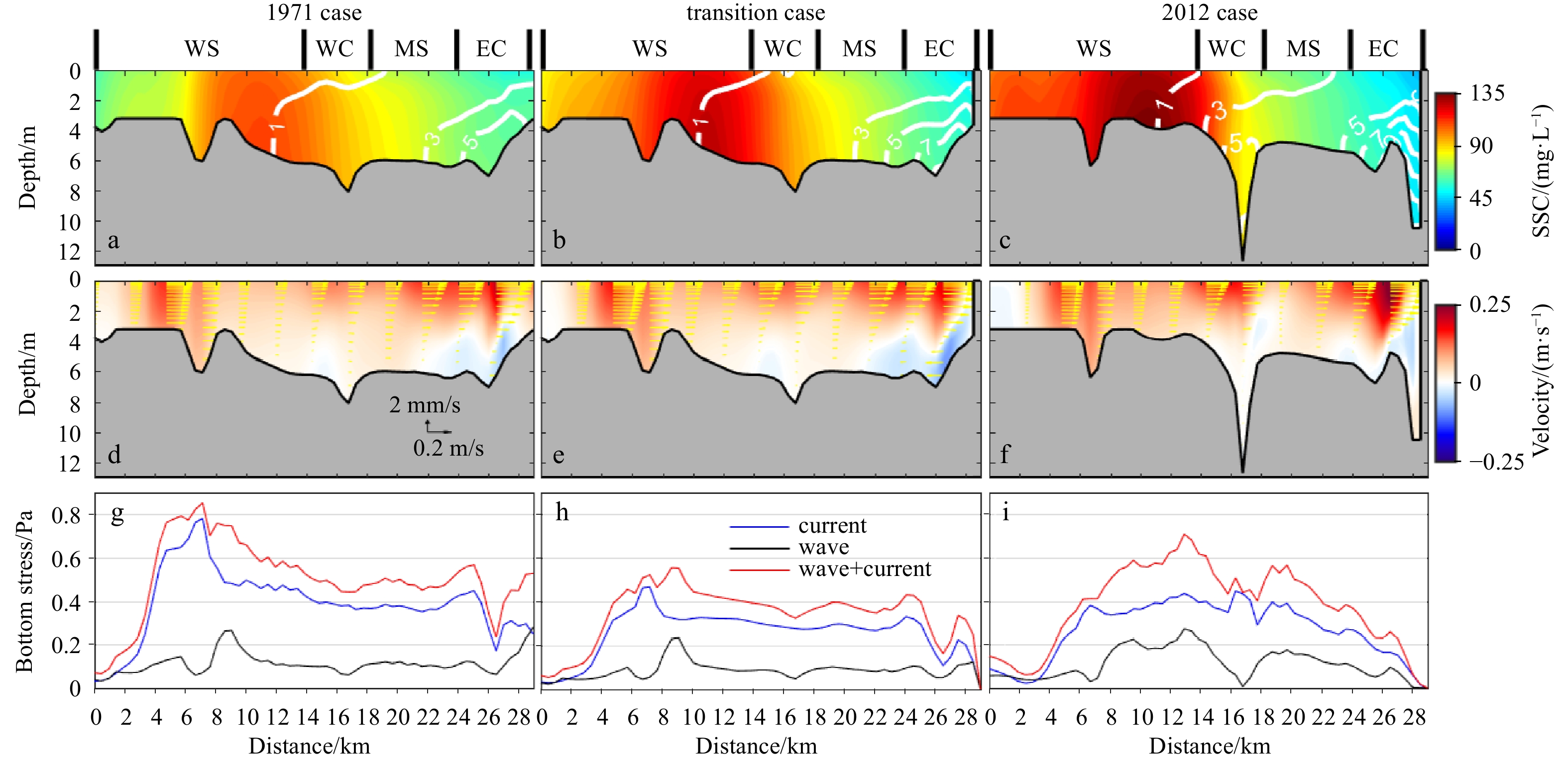
Figure 12. Cross-channel distributions of tidally averaged SSC (contours) and salinity (white lines) (a, b, c), cross-channel residual current (contours and arrows) (d, e, f), and bottom stress (g, h, i) at Section B (shown in Fig. 1e) in spring tide. In a−c, the isohalines are plotted every 2 psu. The positive value for the cross-channel residual current is eastward. The current-induced, wave-induced and wave-current combined bottom stresses are denoted by blue, dark, and red lines, respectively. The 0 km on the x-axis is from the west, and the vantage point is looking in the estuary. The 1971, transition, and 2012 cases are indicated in the left, middle and right panels, respectively.
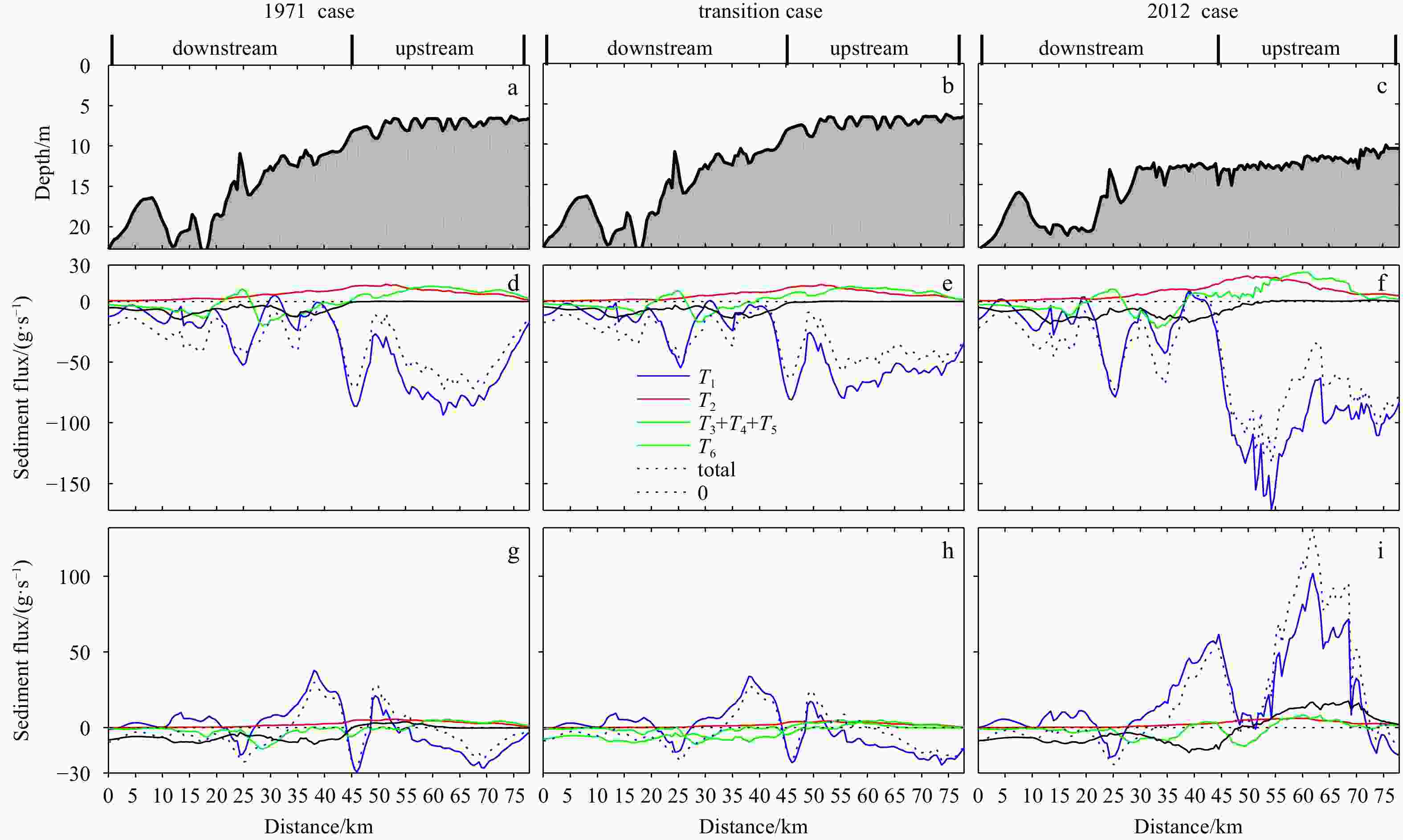
Figure 13. Along-channel bottom bathymetries (a, b, c) and along-channel distributions of tidally averaged sediment fluxes in spring tide (d, e, f) and neap tide (g, h, i) at Section A (shown in Fig. 1e). T1, T2, T3+T4+T5, and T6 represent Eulerian transport, Stokes transport, tidal pumping transport, and vertical shear transport, respectively.
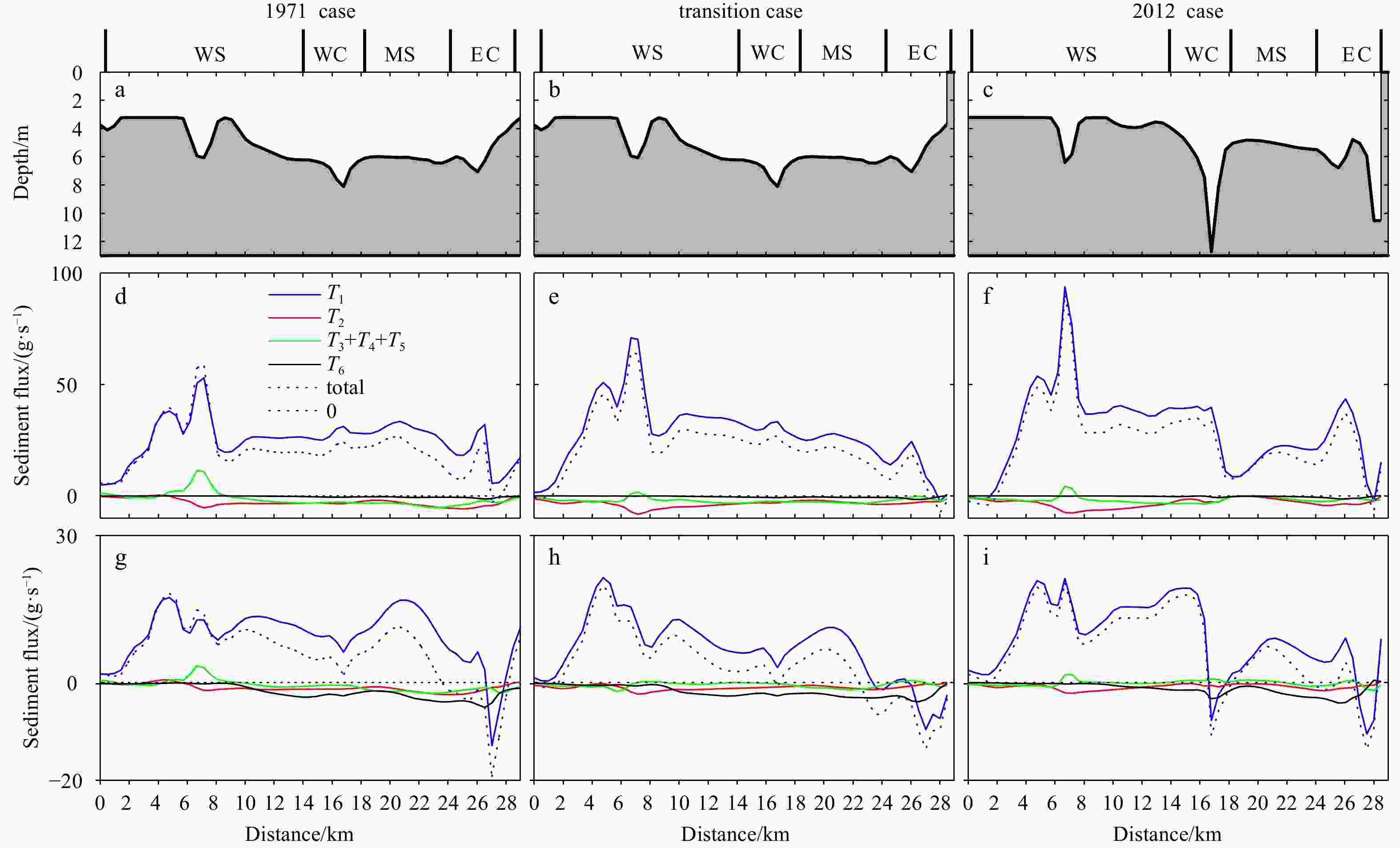
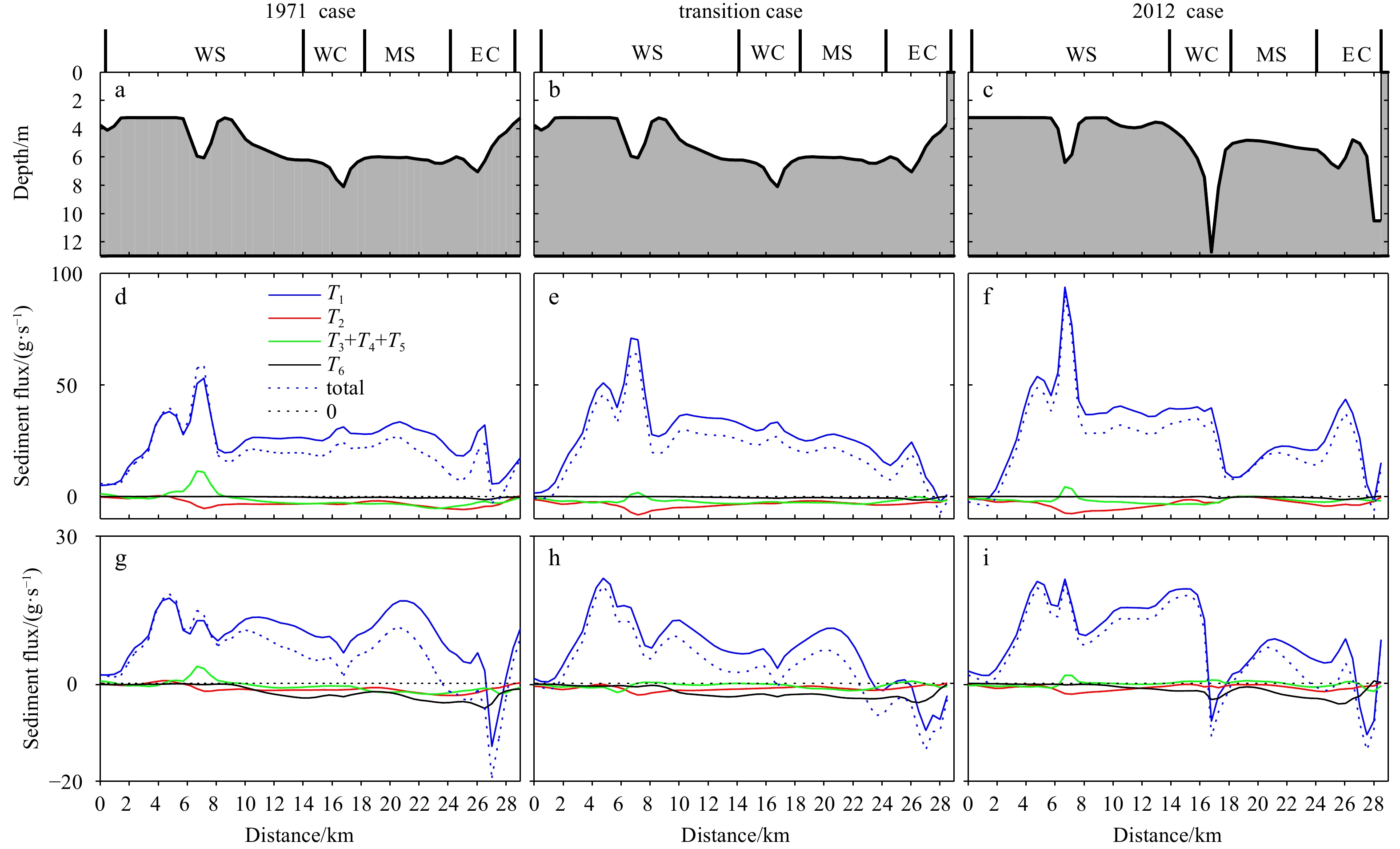
Figure 14. Cross-channel bottom bathymetries (a, b, c) and cross-channel distributions of tidally averaged sediment fluxes in spring tide (d, e, f) and neap tide (g, h, i) at Section B (shown in Fig. 1e). T1, T2, T3+T4+T5, and T6 represent Eulerian transport, Stokes transport, tidal pumping transport, and vertical shear transport, respectively.
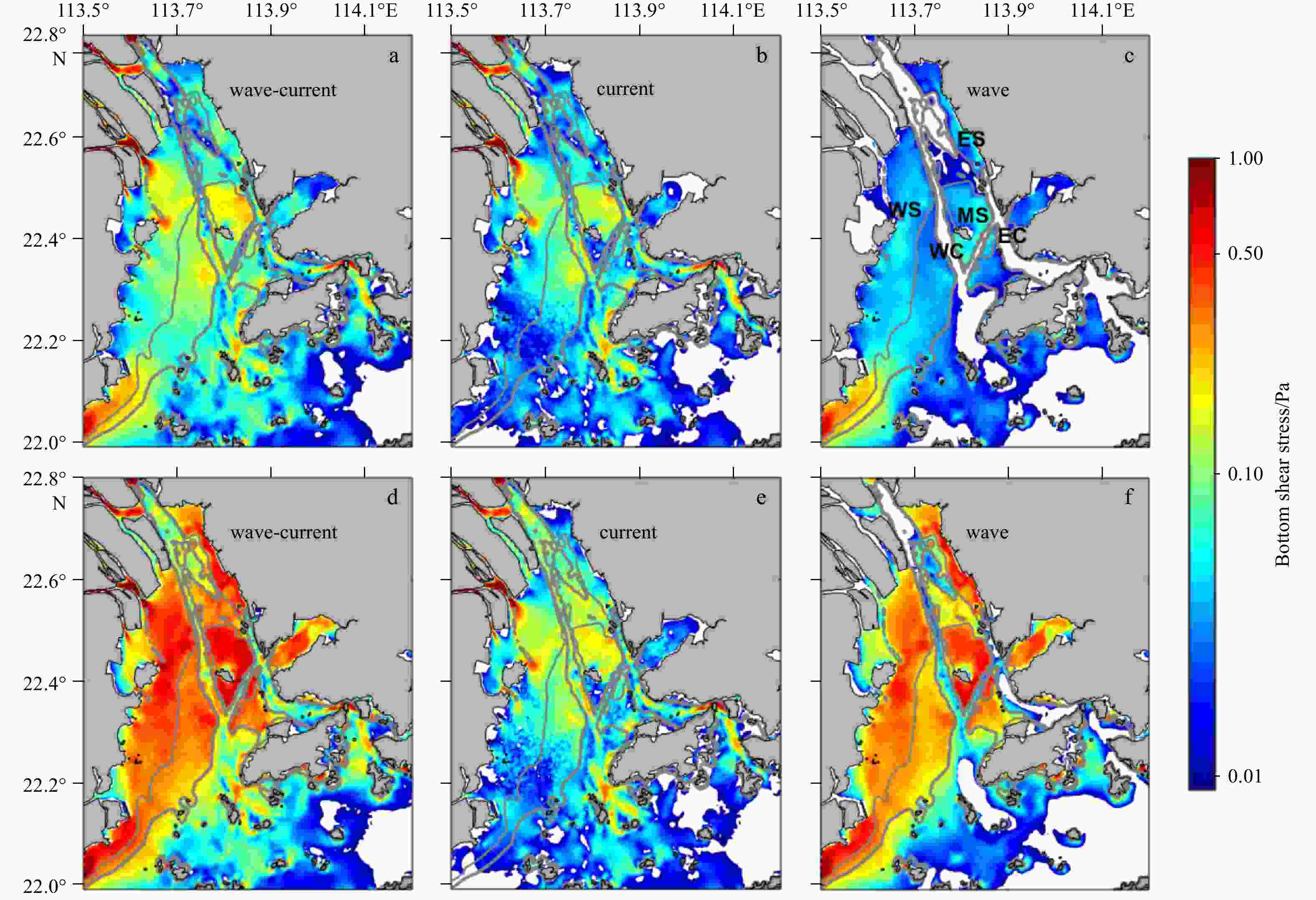
Figure 15. Model results in spring tide in the 2012 case. Tidally averaged bottom stress during the calm period: a. wave-current combined, b. current-induced, c. wave-induced, and during the wavy period: d. wave-current combined, e. current-induced, f. wave-induced. The white areas correspond to bottom stress below 0.01 Pa. Thin/thick gray lines denote 6 m/8 m isobaths.

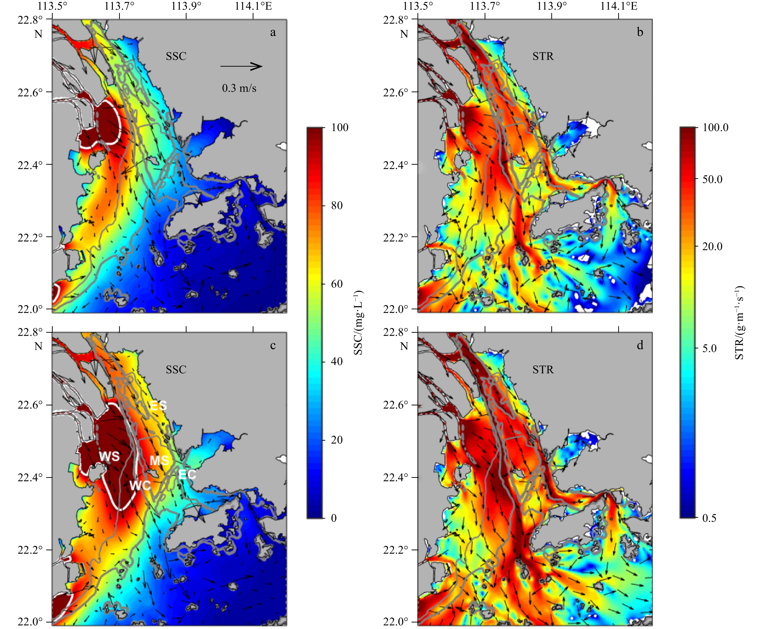
Figure 16. Model results in spring tide in the 2012 case. Tidally and vertically averaged SSC (contour) and residual current (arrow) during the calm period (a) and wavy period (c). Tidally averaged and depth-integrated sediment transport rate (STR; unit: g/(m·s)) during the calm period (b) and wavy period (d). The arrow indicates the direction of the STR, and the white areas indicate an STR below 0.5 g/(m·s). Thin/thick gray lines denote 6 m/8 m isobaths.
Table 1. Sediment parameter settings
Parameter Value Diameter/μm 8.0 Settling velocity/(mm·s−1) 0.038 7 Critical shear stress/Pa 0.022 Density/(kg·m−3) 2 650 Surface erosion rate/(kg·m−2·s−1) 0.000 002 Porosity 0.672  下载: 导出CSV
Table 2. River runoff ratios at the eight outlets
River outlet HUM JM HQL HEM MDM JTM HTM YM Total Ratio/% 12.1 14.0 13.2 16.2 29.6 3.7 4.9 6.3 100 Note: The eight outlets are labeled by HUM, JM, HQL, HEM, MDM, JTM, HTM, and YM, representing Humen, Jiaomen, Hongqili, Hengmen, Modaomen, Jitimen, Hutiaomen, and Yamen, respectively.
下载: 导出CSV
Table 3. Coastlines and bathymetries of the ZRE in the three model scenarios
Scenario Coastline Bathymetry 1971 case 1971 1971 Transition case 2012 1971 2012 case 2012 2012
下载: 导出CSV
Table 4. Skill scores by comparison of modeled results with observations
Station Parameter SK V1 SSC (surface and bottom) 0.56 V2 SSC (surface and bottom) 0.77 W significant wave height 0.82
下载: 导出CSV
Table 5. Areas with depth-averaged SSC greater than 100 mg/L in spring and neap tides in the three scenarios
Period Model scenarios Area/km2 Spring 1971 case 314.4 transition case 255.9 2012 case 284.3 Neap 1971 case 81.5 transition case 77.0 2012 case 88.3 Note: The spring and neap tide periods are denoted by dark and light gray shadows in Fig. 2c, respectively.
下载: 导出CSV
Table 6. Significant wave height and areas with depth-averaged SSC greater than 100 mg/L during calm and wavy periods in the 2012 case
Period Wave condition Significant wave height/m Area/km2 Spring calm period 0.24 363.3 wavy period 0.65 128.2 Neap calm period 0.20 117.8 wavy period 0.58 38.7 Note: The calm and wavy periods are presented by blue and red shadows in Figs 2e and f, respectively. The spring and neap tide periods are denoted by dark and light gray shadows in Fig. 2c, respectively.
下载: 导出CSV
-
Booij N, Ris R C, Holthuijsen L H. 1999. A third-generation wave model for coastal regions: 1. Model description and validation. Journal of Geophysical Research, 104(C4): 7649–7666. doi: 10.1029/98JC02622 Burchard H, Schuttelaars H M, Ralston D K. 2018. Sediment trapping in estuaries. Annual Review of Marine Science, 10: 371–395. doi: 10.1146/annurev-marine-010816-060535 Chapman D C. 1985. Numerical treatment of cross-shelf open boundaries in a barotropic coastal ocean model. Journal of Physical Oceanography, 15(8): 1060–1075. doi: 10.1175/1520-0485(1985)015<1060:NTOCSO>2.0.CO;2 Chen Yongqin David, Chen Xiaohong. 2008. Modeling transport and distribution of suspended sediments in Pearl River estuary. Journal of Coastal Research, (10052): 163–170. doi: 10.2112/1551-5036-52.sp1.163 Cloern J E. 1987. Turbidity as a control on phytoplankton biomass and productivity in estuaries. Continental Shelf Research, 7(11–12): 1367–1381, Dai Zhijun, Fagherazzi S, Mei Xuefei, et al. 2016. Linking the infilling of the north branch in the Changjiang (Yangtze) estuary to anthropogenic activities from 1958 to 2013. Marine Geology, 379: 1–12. doi: 10.1016/j.margeo.2016.05.006 Dai Zhijun, Liu J T, Fu Gui, et al. 2013. A thirteen-year record of bathymetric changes in the north passage, Changjiang (Yangtze) estuary. Geomorphology, 187: 101–107. doi: 10.1016/j.geomorph.2013.01.004 Dai Zhijun, Mei Xuefei, Darby S E, et al. 2018. Fluvial sediment transfer in the Changjiang (Yangtze) river-estuary depositional system. Journal of Hydrology, 566: 719–734. doi: 10.1016/j.jhydrol.2018.09.019 Dai S B, Yang S L, Cai A M. 2008. Impacts of dams on the sediment flux of the Pearl River, southern China. CATENA, 76(1): 36–43. doi: 10.1016/j.catena.2008.08.004 de Jonge V N, Schuttelaars H M, van Beusekom J E E, et al. 2014. The influence of channel deepening on estuarine turbidity levels and dynamics, as exemplified by the Ems estuary. Estuarine, Coastal and Shelf Science, 139: 46–59, Dijkstra Y M, Schuttelaars H M, Schramkowski G, et al. 2019. Modeling the transition to high sediment concentrations as a response to channel deepening in the Ems River Estuary. Journal of Geophysical Research, 124(3): 1578–1594. doi: 10.1029/2018JC014367 Dyer K R. 1974. The salt balance in stratified estuaries. Estuarine and Coastal Marine Science, 2(3): 273–281. doi: 10.1016/0302-3524(74)90017-6 Egbert G D, Erofeeva S Y. 2002. Efficient inverse modeling of Barotropic Ocean tides. Journal of Atmospheric and Oceanic Technology, 19(2): 183–204. doi: 10.1175/1520-0426(2002)019<0183:EIMOBO>2.0.CO;2 Flather R A. 1976. A tidal model of the Northwest European continental shelf. Memoires de la Societe Royale des Sciences de Liege, 6(10): 141–164 Haidvogel D B, Arango H, Budgell W P, et al. 2008. Ocean forecasting in terrain-following coordinates: formulation and skill assessment of the Regional Ocean Modeling System. Journal of Computational Physics, 227(7): 3595–3624. doi: 10.1016/j.jcp.2007.06.016 Hu Jiatang, Li Shiyu, Geng Bingxu. 2011. Modeling the mass flux budgets of water and suspended sediments for the river network and estuary in the Pearl River Delta, China. Journal of Marine Systems, 88(2): 252–266. doi: 10.1016/j.jmarsys.2011.05.002 Kalnay E, Kanamitsu M, Kistler R, et al. 1996. The NCEP/NCAR 40-year reanalysis project. Bulletin of the American Meteorological Society, 77(3): 437–472. doi: 10.1175/1520-0477(1996)077<0437:TNYRP>2.0.CO;2 Kerner M. 2007. Effects of deepening the Elbe Estuary on sediment regime and water quality. Estuarine, Coastal and Shelf Science, 75(4): 492–500, Lesourd S, Lesueur P, Brun-Cottan J C, et al. 2001. Morphosedimentary evolution of the macrotidal Seine estuary subjected to human impact. Estuaries, 24(6): 940. doi: 10.2307/1353008 Lin Shicheng, Liu Guangping, Niu Jianwei, et al. 2021. Responses of hydrodynamics to changes in shoreline and bathymetry in the Pearl River Estuary, China. Continental Shelf Research, 229: 104556. doi: 10.1016/j.csr.2021.104556 Liu Guangping, Cai Shuqun. 2019. Modeling of suspended sediment by coupled wave-current model in the Zhujiang (Pearl) River Estuary. Acta Oceanologica Sinica, 38(7): 22–35. doi: 10.1007/s13131-019-1455-3 Liu Feng, Hu Shuai, Guo Xiaojuan, et al. 2018. Recent changes in the sediment regime of the Pearl River (South China): causes and implications for the Pearl River Delta. Hydrological Processes, 32(12): 1771–1785. doi: 10.1002/hyp.11513 Liu Jintao, Hu Jiatang, Li Shiyu, et al. 2020. A model study on the short-term impact of reclamation on the hydrodynamic processes in the Lingdingyang Bay. Marine Science Bulletin, 39(02): 178–190. doi: 10.11840/j.issn.1001-6392.2020.02.005 Liu Yonggang, MaCcready P, Hickey B M, et al. 2009. Evaluation of a coastal ocean circulation model for the Columbia River plume in summer 2004. Journal of Geophysical Research, 114(C2): C00B04. doi: 10.1029/2008JC004929 Luo Xianlin, Yang Qingshu, Jia Liangwen, et al. 2002. River-bed Evolution of the Pearl River Delta (in Chinese). Guangzhou: Sun Yat-sen University Press, 91–206 Meade R H. 1969. Landward transport of bottom sediments in estuaries of the Atlantic coastal plain. Journal of Sedimentary Research, 39(1): 222–234. doi: 10.1306/74D71C1C-2B21-11D7-8648000102C1865D Mellor G L, Yamada T. 1982. Development of a turbulence closure model for geophysical fluid problems. Reviews of Geophysics, 20(4): 851–875. doi: 10.1029/RG020i004p00851 Orlanski I. 1976. A simple boundary condition for unbounded hyperbolic flows. Journal of Computational Physics, 21(3): 251–269. doi: 10.1016/0021-9991(76)90023-1 Shchepetkin A F, McWilliams J C. 2005. The regional oceanic modeling system (ROMS): a split-explicit, free-surface, topography-following-coordinate oceanic model. Ocean Modelling, 9(4): 347–404. doi: 10.1016/j.ocemod.2004.08.002 Shen Huanting, He Songling, Mao Zhichang, et al. 2001. On the turbidity maximum in the Chinese estuaries. Journal of Sediment Research (in Chinese), (1): 23–29. doi: 10.3321/j.issn:0468-155X.2001.01.004 Song Yuhe, Haidvogel D. 1994. A semi-implicit ocean circulation model using a generalized topography-following coordinate system. Journal of Computational Physics, 115(1): 228–244. doi: 10.1006/jcph.1994.1189 Styles R, Glenn S M. 2000. Modeling stratified wave and current bottom boundary layers on the continental shelf. Journal of Geophysical Research, 105(10): 24119–24139. doi: 10.1029/2000JC900115 Tan Chao, Huang Bensheng, Liu Kunsong, et al. 2017. Using the wavelet transform to detect temporal variations in hydrological processes in the Pearl River, China. Quaternary International, 440: 52–63. doi: 10.1016/j.quaint.2016.02.043 van der Wal D, Pye K, Neal A. 2002. Long-term morphological change in the Ribble Estuary, northwest England. Marine Geology, 189(3/4): 249–266, van Maren D S, van Kessel T, Cronin K, et al. 2015. The impact of channel deepening and dredging on estuarine sediment concentration. Continental Shelf Research, 95: 1–14. doi: 10.1016/j.csr.2014.12.010 Wai O W H, Wang C H, Li Y S, et al. 2004. The formation mechanisms of turbidity maximum in the Pearl River Estuary, China. Marine Pollution Bulletin, 48(5–6): 441–448, Warner J C, Sherwood C R, Signell R P, et al. 2008. Development of a three-dimensional, regional, coupled wave, current, and sediment-transport model. Computers & Geosciences, 34(10): 1284–1306. doi: 10.1016/j.cageo.2008.02.012 Willmott C J. 1981. On the validation of models. Physical Geography, 2(2): 184–194. doi: 10.1080/02723646.1981.10642213 Wei Xing, Cai Shuqun, Zhan Weikang, et al. 2021. Changes in the distribution of surface sediment in Pearl River Estuary, 1975–2017, largely due to human activity. Continental Shelf Research, 228. doi: 10.1016/j.csr.2021.104538 Wu Z Y, Saito Y, Zhao D N, et al. 2016. Impact of human activities on subaqueous topographic change in Lingding Bay of the Pearl River estuary, China, during 1955–2013. Scientific Reports, 6: 37742. doi: 10.1038/srep37742 Xie Lili, Liu Xia, Yang Qingshu, et al. 2015. Variations of current and sediment transport in Lingding Bay during spring tide in flood season driven by human activities. Journal of Sediment Research (in Chinese), (3): 56–62. doi: 10.16239/j.cnki.0468-155x.2015.03.009 Yan Dong, Song Dehai, Bao Xianwen. 2020. Spring-neap tidal variation and mechanism analysis of the maximum turbidity in the Pearl River Estuary during flood season. Journal of Tropical Oceanography (in Chinese), 39(1): 20–35 Yang Liuzhu, Liu Feng, Gong Wenping, et al. 2019. Morphological response of Lingding Bay in the Pearl River Estuary to human intervention in recent decades. Ocean & Coastal Management, 176: 1–10. doi: 10.1016/j.ocecoaman.2019.04.011 Yao Zhangmin, Wang Yongyong, Li Aiming. 2009. Primary analysis of water distribution ratio variation in main waterway in Pearl River Delta. Pearl River (in Chinese), (2): 43–45, 51 Zeng Xiangming, He Ruoying, Xue Zuo, et al. 2015. River-derived sediment suspension and transport in the Bohai, Yellow, and East China Seas: a preliminary modeling study. Continental Shelf Research, 111: 112–125. doi: 10.1016/j.csr.2015.08.015 Zhan Weikang, Wu Jie, Wei Xing, et al. 2019. Spatio-temporal variation of the suspended sediment concentration in the Pearl River Estuary observed by MODIS during 2003–2015. Continental Shelf Research, 172: 22–32. doi: 10.1016/j.csr.2018.11.007 Zhang Guang, Chen Yuren, Cheng Weicong, et al. 2021a. Wave effects on sediment transport and entrapment in a channel-shoal estuary: the Pearl River Estuary in the dry winter season. Journal of Geophysical Research, 126(4): e2020JC016905. doi: 10.1029/2020JC016905 Zhang Guang, Cheng Weicong, Chen Lianghong, et al. 2019. Transport of riverine sediment from different outlets in the Pearl River Estuary during the wet season. Marine Geology, 415: 105957. doi: 10.1016/j.margeo.2019.06.002 Zhang Ping, Yang Qingshu, Wang Heng, et al. 2021b. Stepwise alterations in tidal hydrodynamics in a highly human-modified estuary: the roles of channel deepening and narrowing. Journal of Hydrology, 597: 126153. doi: 10.1016/j.jhydrol.2021.126153 -


 点击查看大图

计量
- 文章访问数: 561
- HTML全文浏览量: 190
- PDF下载量: 30
- 被引次数: 0