

Basis functions for shallow-water temperature profiles based on the internal-wave eigenmodes
-
Abstract: The shallow-water temperature profile is typically parameterized using a few empirical orthogonal function (EOF) coefficients. However, when the experimental area is poorly known or highly variable, the adaptability of the EOFs will be significantly reduced. In this study, a new set of basis functions, generated by combining the internal-wave eigenmodes with the average temperature gradient, is developed for characterizing the temperature perturbations. Temperature profiles recorded by a thermistor chain in the South China Sea in 2015 are processed and analyzed. Compared to the EOFs, the new set of basis functions has higher reconstruction accuracy and adaptability; it is also more stable in ocean regions that have internal waves.
-
Key words:
- temperature profile /
- basis function /
- internal-wave eigenmode /
- EOF /
- sound speed profile
-

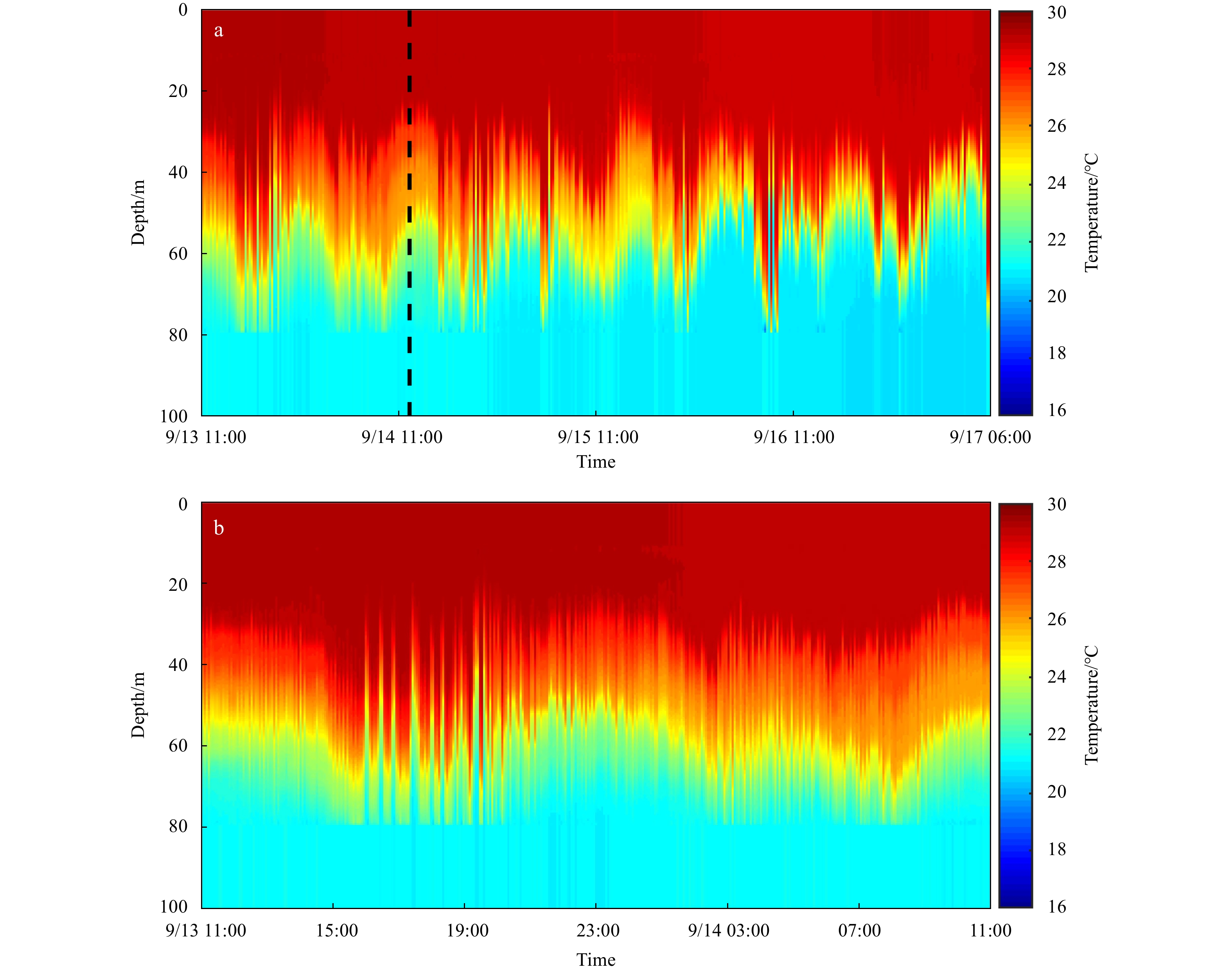
Figure 1. The experimental temperature data. a. The whole temperature profiles from September 13, 11:00 to September 17, 06:00 (GTM), recorded every 30 s. The data on the left of the black dotted line is the training set, and the data on the right of the black dotted line is the test set. b. The temperature training set.

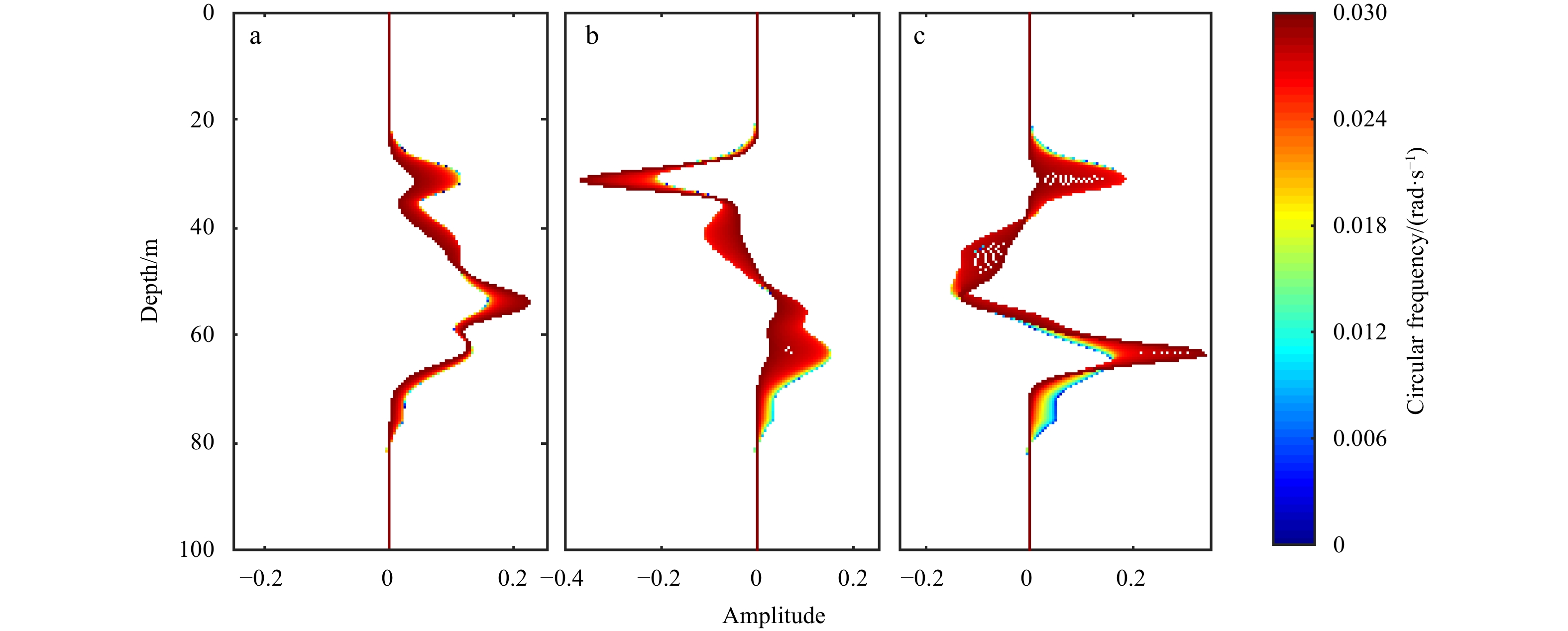
Figure 3. The mean reconstruction error by the IWM11 in different frequency, together with an overlay of the mean value over depth.

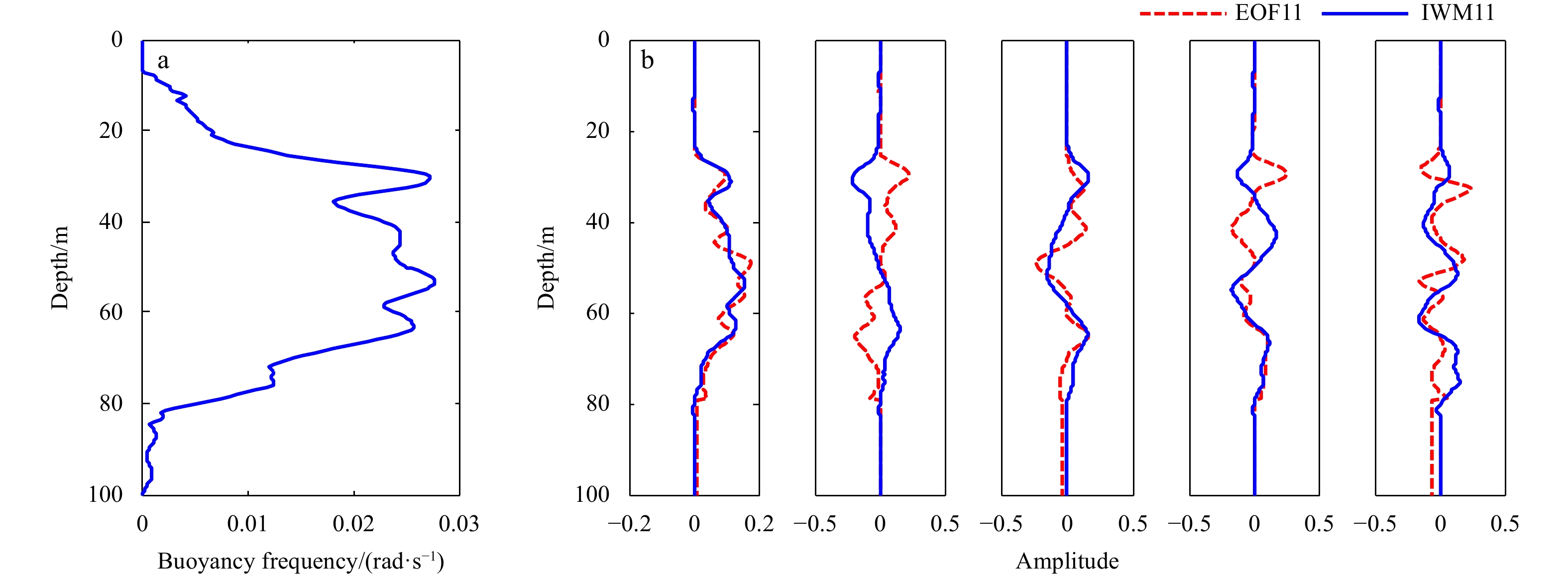
Figure 4. The buoyancy frequency profile (a) and the comparison of the first five modes of the two basis functions (b). The solid blue line represents the IWM11, and the dotted red line represents the EOF11.

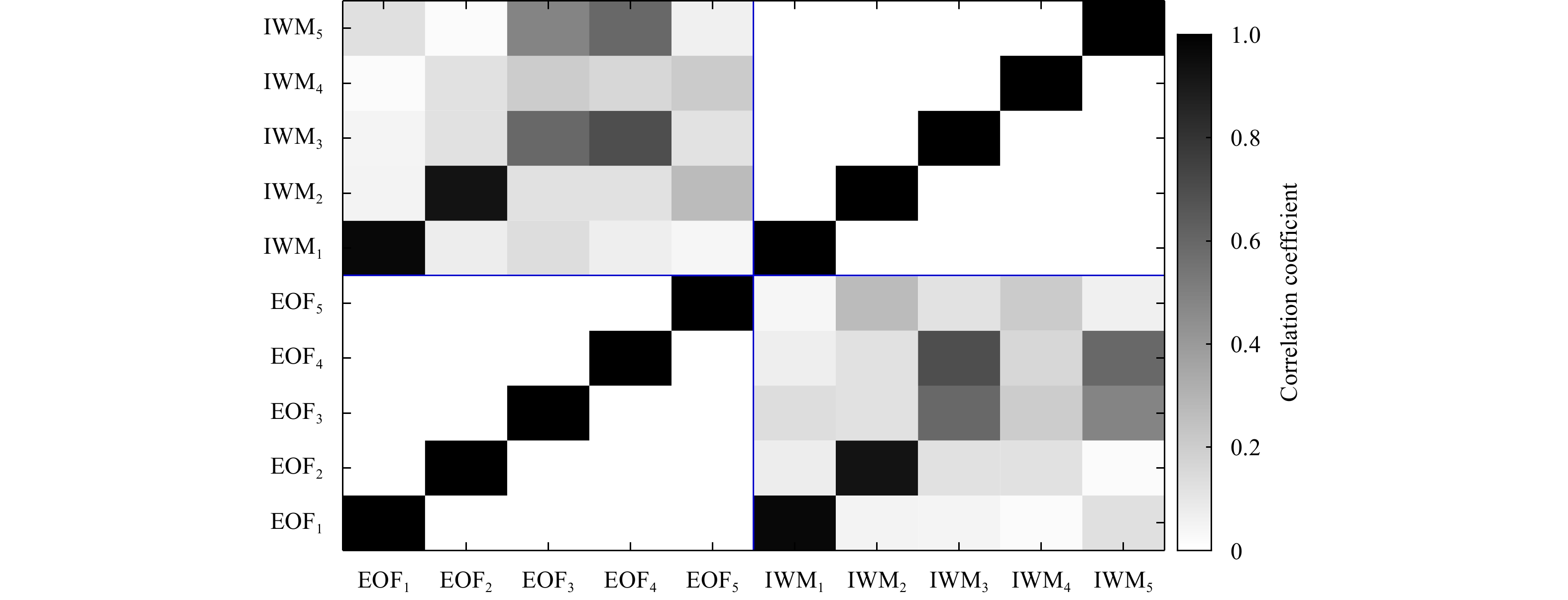
Figure 5. The absolute correlation coefficients between the first five EOF11 and the IWM11 modes.
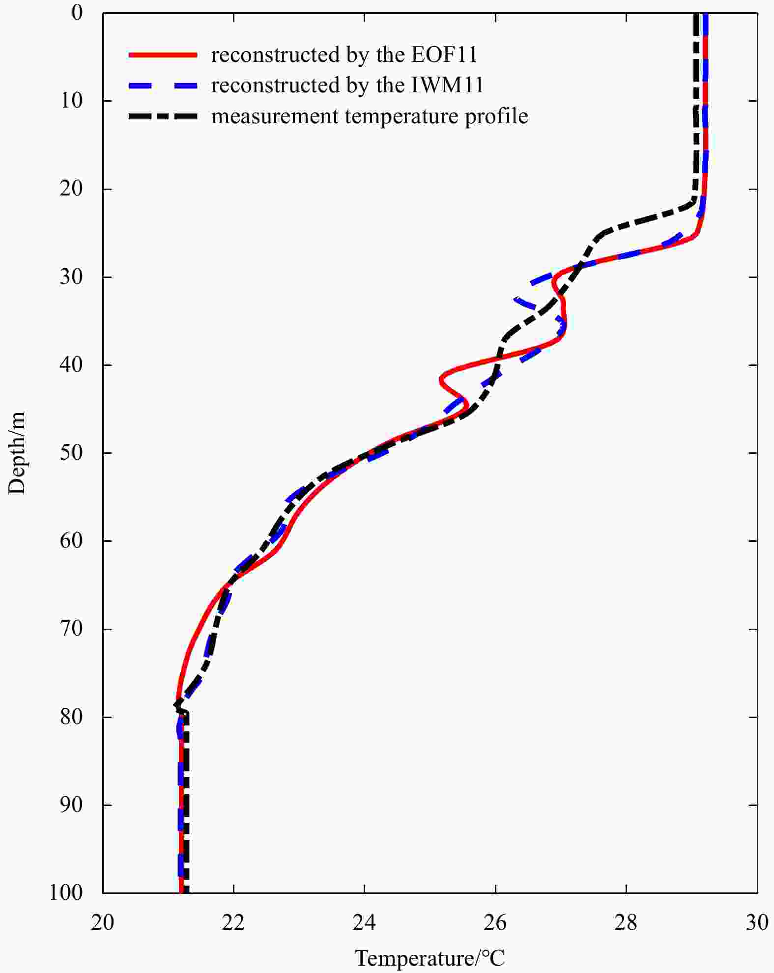
Figure 6. The reconstruction of a randomly selected temperature profile by five coefficients. The black dotted line represents the measurement temperature profile, the red line represents the reconstruction results by the EOF11, and the blue dotted line represents the reconstruction results by the IWM11.
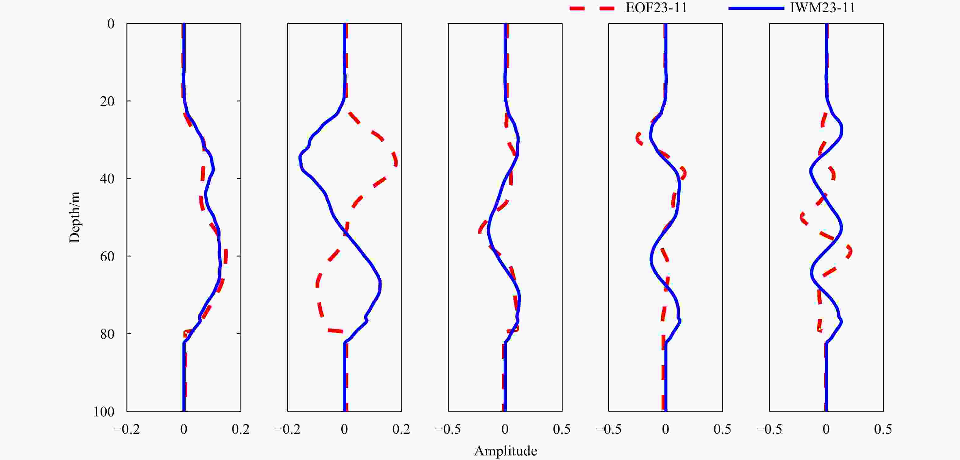
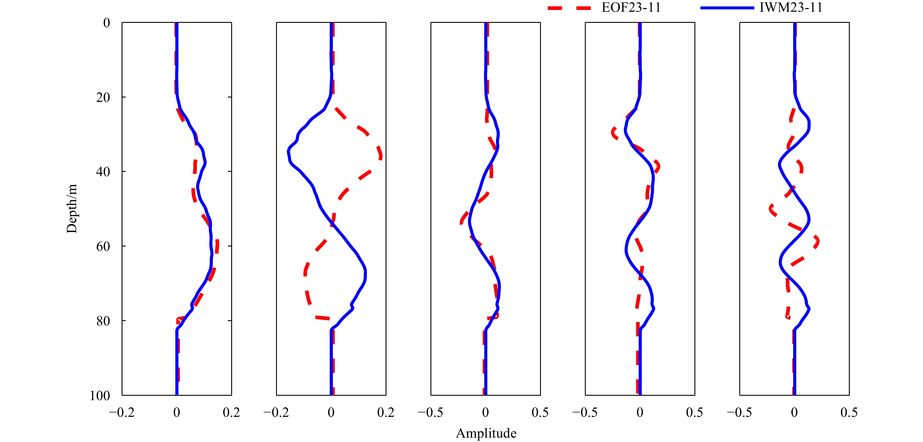
Figure 7. The comparison of the first five modes of the two basis functions. The solid blue line represents the IWM23-11, and the dotted red line represents the EOF23-11.

Figure 8. The absolute correlation coefficient between the first five modes of the EOF23-11 and the IWM23-11.
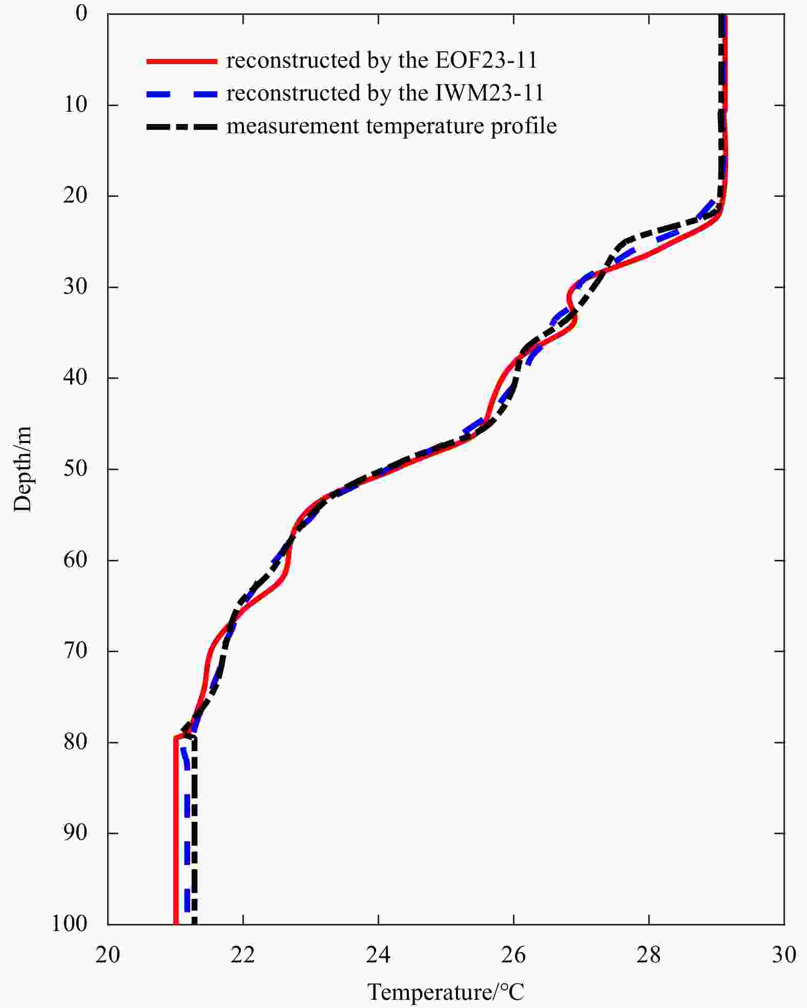
Figure 9. The reconstruction of the selected temperature profile using five coefficients. The black dotted line represents the measurement temperature profile, the red line represents the reconstruction results using the EOF23-11, and the blue dotted line represents the reconstruction results using the IWM23-11.

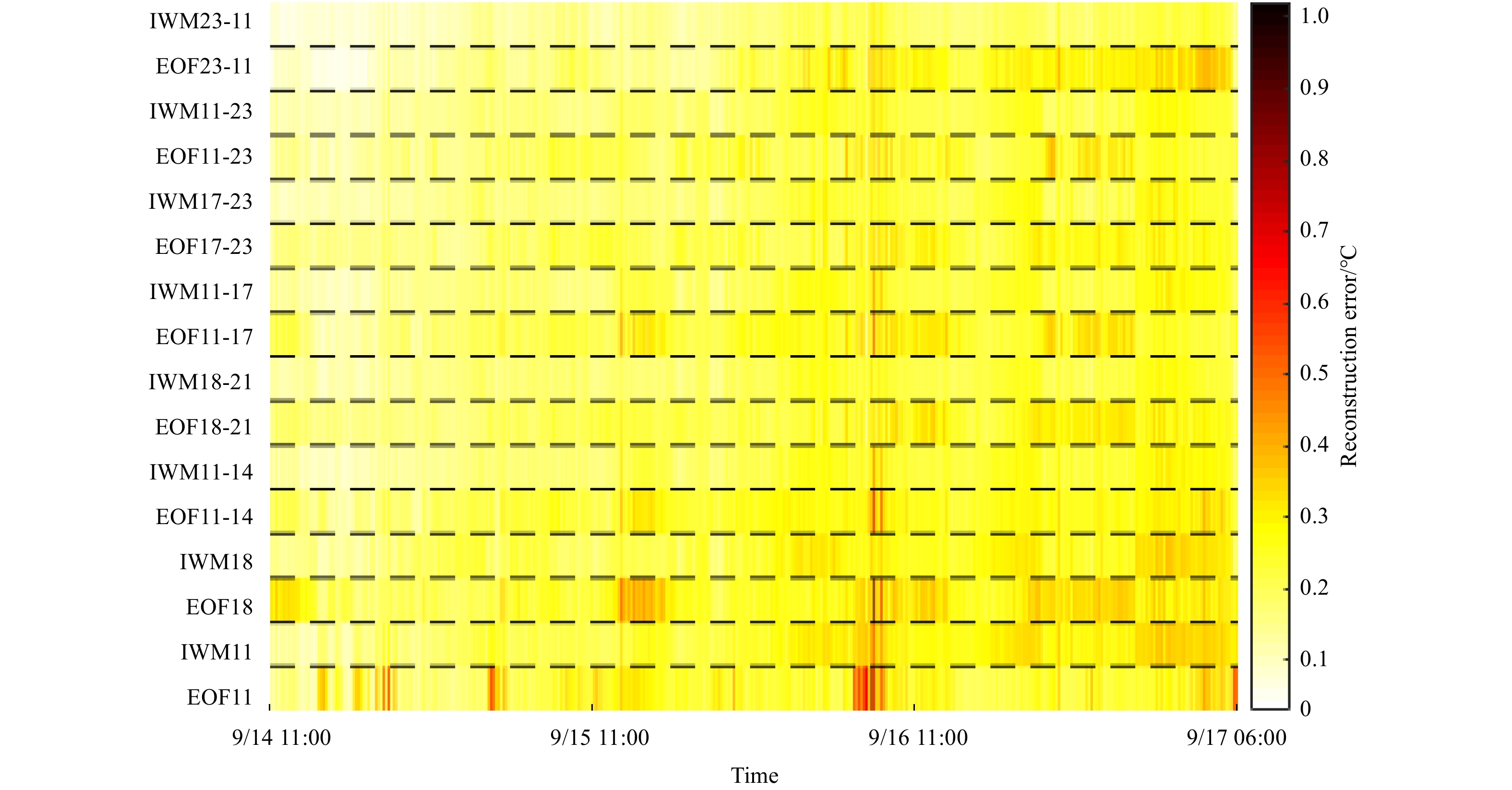
Figure 10. The reconstruction mean error of the temperature profiles in the test set with the 16 sets of basis functions.
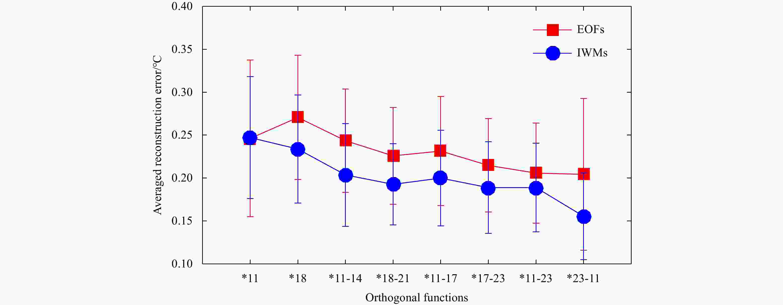
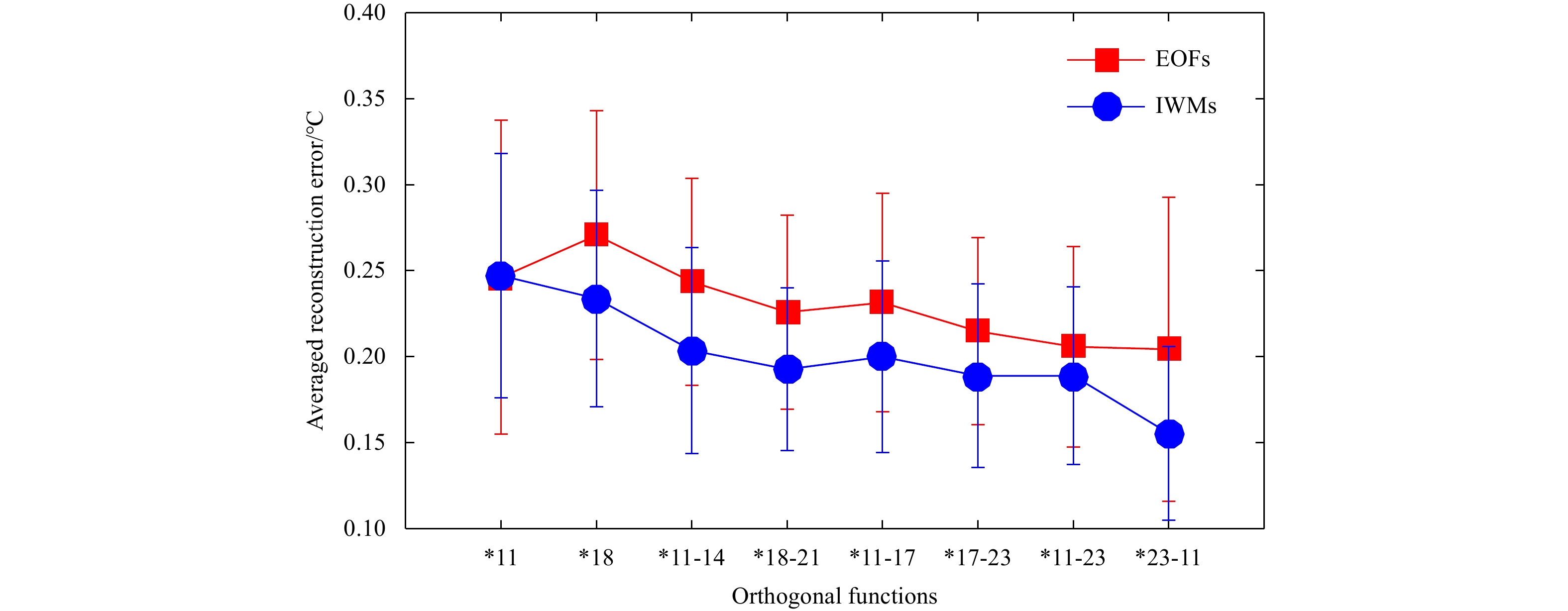
Figure 11. The average reconstruction errors using the 16 different basis functions. The red square represents the average reconstruction errors using the EOFs, and the blue circular represents the average reconstruction errors using the IWMs. The length of the vertical line represents the standard deviation. * represents EOF or IWM.
-
Apel J R. 1987. Principles of Ocean Physics. San Diego, CA: Academic Press, 61–121 Jensen F B, Kuperman W A, Porter M B, et al. 2011. Computational Ocean Acoustics. 2nd ed. New York: Springer, 3–10 Kakatkar R, Gnanaseelan C, Chowdary J S. 2020. Asymmetry in the Tropical Indian Ocean subsurface temperature variability. Dynamics of Atmospheres and Oceans, 90: 101142. doi: 10.1016/j.dynatmoce.2020.101142 Li Zhenglin, He Li, Zhang Renhe, et al. 2015. Sound speed profile inversion using a horizontal line array in shallow water. Science China Physics, Mechanics & Astronomy, 58(1): 1–7 Li Qianqian, Shi Juan, Li Zhenglin, et al. 2019a. Acoustic sound speed profile inversion based on orthogonal matching pursuit. Acta Oceanologica Sinica, 38(11): 149–157. doi: 10.1007/s13131-019-1505-4 Li Fenghua, Wang Kai, Yang Xishan, et al. 2021. Passive ocean acoustic thermometry with machine learning. Applied Acoustics, 181: 108167. doi: 10.1016/j.apacoust.2021.108167 Li Fenghua, Yang Xishan, Zhang Yanjun, et al. 2019b. Passive ocean acoustic tomography in shallow water. The Journal of the Acoustical Society of America, 145(5): 2823–2830. doi: 10.1121/1.5099350 Monahan A H, Fyfe J C, Ambaum M H P, et al. 2009. Empirical orthogonal functions: the medium is the message. Journal of Climate, 22(24): 6501–6514. doi: 10.1175/2009JCLI3062.1 Song Wenhua, Hu Tao, Guo Shengming, et al. 2014. A methodology to achieve the basis function for the expansion of sound speed profile. Chinese Journal of Acoustics, 33(3): 299–311 Tan B A, Gerstoft P, Yardim C, et al. 2013. Broadband synthetic aperture geoacoustic inversion. The Journal of the Acoustical Society of America, 134(1): 312–322. doi: 10.1121/1.4807567 Tielbürger D, Finette S, Wolf S. 1997. Acoustic propagation through an internal wave field in a shallow water waveguide. The Journal of the Acoustical Society of America, 101(2): 789–808. doi: 10.1121/1.418039 -

 下载:
下载:


 点击查看大图
计量
- 文章访问数: 273
- HTML全文浏览量: 86
- PDF下载量: 11
- 被引次数: 0