


Figure
1.
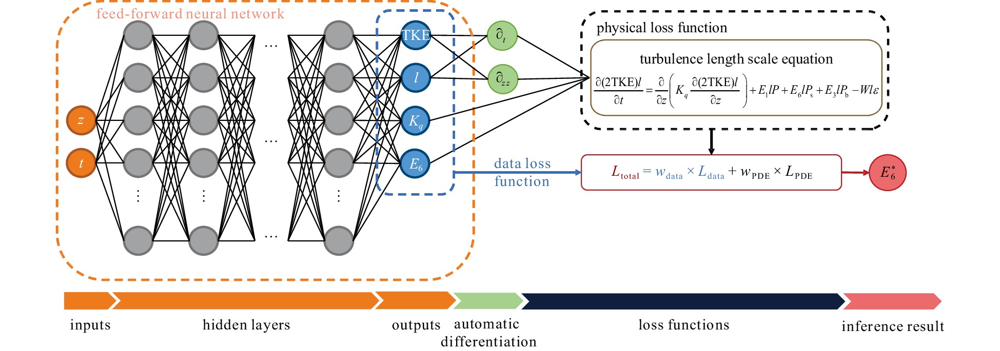
Architecture of physical-informed neural network for key parameter E6 inference in KC04. TKE, turbulent kinetic energy.
| Citation: | Fangrui Xiu, Zengan Deng. Performance of physical-informed neural network (PINN) for the key parameter inference in Langmuir turbulence parameterization scheme[J]. Acta Oceanologica Sinica, 2024, 43(5): 121-132. doi: 10.1007/s13131-024-2329-4

|
Langmuir circulation (LC), which results from the interplay between Stokes drift and mean flow (Craik and Leibovich, 1976; Suzuki and Fox-Kemper, 2016), induces Langmuir turbulence (LT) and exerts a substantial influence on the dynamics of the upper ocean (Cao et al., 2019). To depict the additional mixing induced by the LT in the Reynold-Averaged Numerical Simulation (RANS) model, Kantha and Clayson (2004) (KC04) integrated a Stokes-Euler cross-shear production (Ps) into the Mellor-Yamada type (MY-type) closure scheme (Kantha and Clayson, 1994; Mellor and Yamada, 1974, 1982). This integration affected both the turbulent kinetic energy (TKE) and turbulent length scale equations. Building upon the KC04 scheme, Harcourt (2013, 2015) (H13, H15) introduced the Craik-Leibovich vortex force (Craik and Leibovich, 1976) into algebraic Reynolds stress models. This inclusion addressed the influence of LC on the stability functions, TKE, and turbulent length scale equations, with the aim of optimizing the LT parameterization scheme. To achieve this optimization, the KC04, H13, and H15 schemes all incorporated the Stokes production coefficient (E6) in the turbulent length scale equation, scaling the LT effect.
Despite the critical role of E6 in the MY-type LT parameterization scheme, a standardized methodology for its inference remains elusive. In the KC04 scheme, E6 was initially set to 4.0 by Kantha and Clayson (2004) before being adjusted to 7.2 by Kantha et al. (2010). Harcourt (2015) modified E6 to 6.0 in the H15 scheme to address excessively high intermediate layer maxima and enhance simulations in ideal cases. Unfortunately, these E6 values were selected based on experiential knowledge and comparative experiments, potentially needing more accuracy in representing realistic turbulent conditions (Martin and Savelyev, 2017). Meanwhile, these fixed values make the RANS results subject to some error compared to the results of more accurate large eddy simulations (LES) in various wind and wave conditions (Harcourt, 2013, 2015). It is evident that the performance of RANS models is notably sensitive to the selection of empirical parameters, highlighting the challenges associated with parameter choices (Xiao and Cinnella, 2018). Given the inherent complexity of non-linear partial differential equations (PDEs) in turbulent systems, developing a robust method for accurately inferring the optimal value of E6 to improve the MY-type LT parameterization schemes remains an urgent scientific concern. Since the KC04 scheme is the basis in the MY-type LT parameterization schemes, it was decided to use the KC04 scheme as the object in this study to explore the method of inferring the E6 in it, which could provide more informative and meaningful results for the study of LT parameterization schemes including H13 and H15, etc.
Traditional methods for inferring and estimating empirical parameters in RANS models include the ensemble Kalman filter (Kato and Obayashi, 2012), evolution methods (Gimenez and Bre, 2019), and Bayesian inference (Doronina et al., 2020; Hemchandra et al., 2023). However, these methods may not fully incorporate explicit physical constraints during the parameter inference process. This limitation becomes particularly critical in complex nonlinear problems, like handling high-dimensional issues and sensitivity to local optima, especially in scenarios demanding strict adherence to physical laws. In this context, the physics-informed neural network (PINN) offers a groundbreaking approach. Distinguished by its integration of deep learning with physical constraints in loss functions, PINN ensures accurate learning of input-output mappings while strictly adhering to pertinent physical laws (Raissi et al., 2019). Crucially, PINN has demonstrated its capability to maintain physical consistency and effective learning even in data-limited scenarios, a notable challenge for traditional methods (Bajaj et al., 2023; Xu et al., 2023). PINN, on the other hand, through its meshless nature, can fit the governing PDEs directly in continuous space, effectively avoiding the errors and complexities that may be introduced by traditional discretization methods, which is particularly critical for capturing the complex dynamics of turbulent flow fields (Abueidda et al., 2021; Raissi et al., 2019; Raissi and Karniadakis, 2018). These allow it to be used as a complement to traditional methods to solve inverse problems in highly nonlinear problems. When using PINN to solve inverse problems, constraint data plays an indispensable role. The constraint data, even if limited and possibly noisy, is essential for accurately deducing unknown parameters in the governing PDEs. Constrained by the given data and PDEs, PINN can accurately model and reflect the actual behavior of physical systems in the solution domain, ensuring that the inferred values of parameters are not only theoretically sound but also practically accurate.
The efficacy and accuracy of PINN in various tasks related to parameter inference in RANS models have been thoroughly validated. For instance, PINN has demonstrated the accurate inference of roughness parameters in one-dimensional differential equations (Cedillo et al., 2022) and the optimization of empirical parameters in k-ε closure schemes (Luo et al., 2020). Nonetheless, it is crucial to emphasize that a specific configuration effective for one set of equations in PINN may not necessarily yield similar results for others (Raissi et al., 2019). Additionally, there is currently no empirical evidence to support the effective inference of LT-related parameters in MY-type parameterization schemes using PINN. Therefore, this study aimed to assess the feasibility and accuracy of E6 inference using PINN based on the classical KC04 scheme. The selection of an activation function holds paramount importance in ensuring the reliability and precision of a PINN, particularly when conferring non-linear properties (Abbasi and Andersen, 2023; Ramachandran et al., 2018). Smoother activation functions (e.g., hyperbolic tangent and sine function) outperform non-smooth activation functions (e.g., ReLU) in PINN (Zhang et al., 2022). However, the choice of activation function is contingent on the specific task at hand (Jagtap et al., 2020). Additionally, as a numerical approach, PINN is significantly affected by the sampling intervals (Krishnapriyan et al., 2021; Wu et al., 2023). Consequently, for the spatiotemporal dependence problem, the experimental selection of appropriate sampling intervals is indispensable.
Given this, this study conducted numerical simulations to examine the response of turbulent variables to variations in E6 using a water column model with the KC04 scheme. This determination established the sampling depth range for the PINN model. Subsequently, the feasibility and accuracy of inferring E6 using the PINN model were evaluated. The impact of two critical hyperparameters, namely, the activation function and spatiotemporal sampling interval of the input data, was also thoroughly investigated. The optimal configuration for employing PINN in this specific task was identified through this comprehensive exploration.
This paper is organized as follows. Section 2 provides an overview of the one-dimensional column model embedded with the KC04 scheme and introduces the PINN architecture for E6 inference. Section 3 outlines two sets of sensitivity experiments, with the first focusing on the numerical sensitivity of modelling turbulent variables to variations in E6. The second set evaluates the feasibility of PINN for the E6 inference task and presents the optimal solution for the two key hyperparameters. Section 4 presents the results of the two experiment sets. Subsequently, Section 5 discusses and analyzes the experimental results, and Section 6 offers a comprehensive summary and outlook.
The primary impact of LT is observed in vertical mixing of the upper ocean (McWilliams and Sullivan, 2000). Therefore, employing a water column model is advantageous for characterizing the vertical variation of each physical variable, facilitating a rational simplification of the associated physical processes. The General Ocean Turbulence Model (GOTM), a widely utilized one-dimensional column model for studying LT parameterization schemes (Li et al., 2019; Umlauf et al., 2006; Umlauf and Burchard, 2005), was employed in this study to simulate the turbulent variables. The GOTM offers a flexible interface for modifying turbulence closure models to solve the closure problems occurring in Reynolds-Averaged equations. In particular, the KC04 scheme introduces Ps into both the TKE equation and the turbulent length scale equation. The KC04 scheme used in this study is shown as
| $$ \frac{{\partial {q^2}}}{{\partial t}} = \frac{\partial }{{\partial z}}\left( {{K_q}\frac{{\partial {q^2}}}{{\partial z}}} \right) + P + {P_{\mathrm{s}}} + {P_{\mathrm{b}}} - \varepsilon , $$ | (1) |
| $$ \frac{{\partial {q^2}l}}{{\partial t}} = \frac{\partial }{{\partial z}}\left( {{K_q}\frac{{\partial {q^2}l}}{{\partial z}}} \right) + {E_1}lP + {E_6}l{P_{\mathrm{s}}} + {E_3}l{P_{\mathrm{b}}} - Wl\varepsilon , $$ | (2) |
where z and t are the spatial and temporal coordinates, respectively; q is the turbulent velocity scale; l is the turbulent length scale; Kq is the vertical diffusivity coefficient for q2 and q2l; W is the Wall function, taking a value of 2.33 near the sea surface; E1 and E3 are model constants, consistent with those used in Martin and Savelyev (2017); E6 is the Stokes production coefficient; and P, Ps, Pb, and ε are the mean flow shear production shown as
| $$ P = {K_{\mathrm{M}}}\left[ {{{\left( {\frac{{\partial u}}{{\partial z}}} \right)}^2} + {{\left( {\frac{{\partial v}}{{\partial z}}} \right)}^2}} \right], $$ | (3) |
and the Stokes-Euler cross-shear production shown as
| $$ P_{\mathrm{s}}=K_{\mathrm{M}}\left(\frac{\partial u}{\partial z}\frac{\partial u^{\mathrm{s}}}{\partial z}+\frac{\partial v}{\partial z}\frac{\partial v^{\mathrm{s}}}{\partial z}\right), $$ | (4) |
and the buoyancy production shown as
| $$ {P_{\mathrm{b}}} = {K_{\mathrm{H}}}\frac{g}{{{\rho _0}}}\frac{{\partial \rho }}{{\partial z}}, $$ | (5) |
and dissipation term shown as
| $$ \varepsilon = \frac{{{q^3}}}{{{b_1}l}}, $$ | (6) |
where b1 is a model constant, consistent with those used in Martin and Savelyev (2017); the TKE was calculated as q2/2; (u, v) and (us, vs) are the east-west and north-south components of the Eulerian mean current and Stokes drift, respectively; KM and KH are the vertical eddy viscosity coefficient and the vertical diffusivity coefficients for tracer, respectively; g corresponds to the gravitational acceleration; ρ is the potential density of seawater; and ρ0 is the reference seawater density. Kq is equal to 0.41KM (Martin and Savelyev, 2017).
Addressing inverse problems inherently involves understanding the form of the differential operator and inferring unknown empirical parameters through a data-driven computational process. The structure of this methodology is shown in Fig. 1, illustrating the PINN architecture proposed by Raissi et al. (2019) for inferring the Stokes production coefficient E6 within the KC04 scheme. At the core of this architecture lies a feed-forward neural network adept at efficiently linking spatiotemporal coordinates with the parameter to be inferred, as well as turbulent variables requiring differential operations. To ensure that the inferred results align accurately with physical laws, necessary physical constraints are established by employing automatic differentiation techniques (Baydin et al., 2017; Paszke et al., 2017; Wengert, 1964).
The state of spatiotemporal evolution of the turbulent variables u(z, t) is considered as a function of the spatiotemporal coordinates. A feed-forward neural network, uNN(z, t; θ), essentially approximates a function comprising NL layers, including one input layer, NL − 2 hidden layers, and one output layer. Therefore, the utilization of uNN(z, t; θ) to approximate u(z, t) can be expressed as presented as
| $$\begin{split} u(z,t) \approx \ &{u^{{\mathrm{NN}}}}(z,t;\theta ) = {W_{{N_{\mathrm{L}}}{{ - 1}}}}\sigma \left( \cdots {W_2}\sigma \left( {{W_1}[z,t] + {b_1}} \right) +\right.\\ &\left.{b_2} \cdots \right) + {b_{{N_{\mathrm{L}}} - 1}}, \end{split}$$ | (7) |
where Wi denotes the weight matrix, bi denotes the bias vector, and the combination of these two forms the learnable parameter matrix θ = [Wi; bi], i denotes the i-th layer of the network, and σ denotes the activation function. The NL layer of the network is the output layer, which is linear and does not need to go through the activation function operation again. To enhance the generalization ability of the model over different solution domains, the input coordinate (z, t) will be first normalized when fed into the network, and the normalization formula is shown as
| $$ \left\{\begin{split}z=2\times\dfrac{z-\min(z)}{\max(z)-\min(z)}-1, \\ t=2\times\dfrac{t-\min(t)}{\max(t)-\min(t)}-1.\end{split}\right. $$ | (8) |
It is important to note that the normalization performed here is done after (z, t) is fed into the network, while it is still the original (z, t) that is involved in the computation when performing the automatic differentiation. To achieve optimal fitting, we constructed a data loss function by incorporating known data at the sampling points, enabling backward propagation for tuning the network parameters. The expression for the data loss function in the PINN is provided as
| $$ L_{\mathrm{data}}=\frac{1}{M\times N}\sum\limits_{j=1}^M\sum\limits_{i=1}^N\left|u^{\mathrm{NN}}\left(z^i,t\; ^j;\theta\right)-u^{i,j}\right|^2, $$ | (9) |
where M is the number of temporal coordinate points, N is the number of spatial coordinate points, i is the i-th spatial coordinate point, and j is the j-th temporal coordinate point.
To ensure the physical constraint and match an optimal fit between the PDE and the known data, a physical loss function constrained by the PDE should be developed. Utilizing the automatic differentiation technique facilitates the acquisition of the partial derivatives of u (z, t; θ). Here,
| $$ G\left( {u,{\partial _z}u,{\partial _t}u, \cdots ,{\partial _{zz}}u, \cdots ,{u^{\mathrm{c}}};z,t,\lambda } \right) = 0, $$ | (10) |
where
| $$ {f\;^{{\mathrm{NN}}}}\left( {z,t;\theta } \right): = G\left( {{u^{{\mathrm{NN}}}},{\partial _z}{u^{{\mathrm{NN}}}},{\partial _t}{u^{{\mathrm{NN}}}}, \cdots ,{\partial _{zz}}{u^{{\mathrm{NN}}}}, \cdots ,{u^{\mathrm{c}}};z,t,\lambda } \right), $$ | (11) |
where uc represents the variables directly provided to structure the physical loss function, eliminating the need for differential operation. Consequently, the physical loss function can be written as
| $$ {L_{{\mathrm{PDE}}}} = \frac{1}{N}{\left| {{f\;^{{\mathrm{NN}}}}\left( {x;\theta } \right)} \right|^2}. $$ | (12) |
Finally, the overall loss function in the PINN comprises both the data loss function and physical constraint loss function shown as
| $$ {L_{{\mathrm{total}}}} = {w_{{\mathrm{data}}}} \times {L_{{\mathrm{data}}}} + {w_{{\mathrm{PDE}}}} \times {L_{{\mathrm{PDE}}}}, $$ | (13) |
where wdata and wPDE are the tunable weights assigned to the data loss function and the physical loss function, respectively (Wight and Zhao, 2020). The inclusion of geometry, boundary conditions, or initial conditions within the loss function is not mandatory. The inferred value
In this study, the feed-forward neural network was fed spatiotemporal coordinates (z, t) as the input. The output layer generates key variables including TKE, l, Kq, and E6. Among these, TKE, l, and Kq are subject to dual constraints, aligning with the data derived from the GOTM as part of the data loss function and adhering to the turbulent scale equation within the physical loss function. In contrast, E6 is regulated solely by the physical loss function. The turbulent length scale equation defined in the KC04 scheme serves as the foundational physical constraint expressed as
| $$ \begin{split}{L_{{\text{KC04}}}} = \ &\frac{{\partial (2{\mathrm{TK}}{{\mathrm{E}}^{{\mathrm{NN}}}}){l^{{\mathrm{NN}}}}}}{{\partial t}} - \frac{\partial }{{\partial z}}\left( {{K_q}^{ {\mathrm{NN}}}\frac{{\partial (2{\mathrm{TK}}{{\mathrm{E}}^{{\mathrm{NN}}}}){l^{{\mathrm{NN}}}}}}{{\partial z}}} \right) -\\ & {E_1}{l^{{\mathrm{NN}}}}P - {E_6}^{ {\mathrm{NN}}}{l^{{\mathrm{NN}}}}{P_{\mathrm{s}}} - {E_3}{l^{{\mathrm{NN}}}}{P_{\mathrm{b}}} + W{l^{{\mathrm{NN}}}}\varepsilon .\end{split} $$ | (14) |
Furthermore, variables such as P, Ps, Pb, and ε were incorporated directly into the physical loss function.
Two sets of experiments were conducted in this study. The first set, designated as the GOTM sensitivity experiment set (Set1), was used to examine the effects of E6 on GOTM simulations. The results of this set inform the selection of the sampling depth range for subsequent experiments. The second set, denoted as the PINN hyperparameters sensitivity experiment set (Set2), encompassed two specific experiments: the activation functions sensitivity experiment (Exp1) and the sampling intervals sensitivityexperiment (Exp2). These experiments were designed to investigate the effects of various activation functions and spatiotemporal sampling intervals of input data on the feasibility and accuracy of the E6 inference. An overview of the experimental framework is listed in Table 1.
| Experimental set (number) | Experiment (number) | Activation function |
Sampling intervals | Preset E6 value (case number)/ model number |
| GOTM sensitivity experiment set (Set1) | / | / | / | 5.0 (Case 1), 6.0 (Case 2), 7.0 (Case 3), 8.0 (Case 4) |
| PINN key hyperparameters sensitivity experiment set (Set2) |
Activation Functions sensitivity experiment (Exp1) |
Tanh | Δt = 1 s, Δz = 0.1 m | Model 1_1 |
| Arctan | Δt = 1 s, Δz = 0.1 m | Model 1_2 | ||
| Sin | Δt = 1 s, Δz = 0.1 m | Model 1_3 | ||
| Sampling intervals sensitivity experiment (Exp2) |
the optimal one in Exp1 |
Δt = 2 s, Δz = 0.1 m | Model 2_1 | |
| Δt = 5 s, Δz = 0.1 m | Model 2_2 | |||
| Δt = 1 s, Δz = 0.2 m | Model 2_3 | |||
| Δt = 1 s, Δz = 0.5 m | Model 2_4 | |||
| Notes: / indicates that the item is not set or used in the experiment set. | ||||
 DownLoad:
CSV
DownLoad:
CSV
Set1 included four distinct cases utilizing preset values of E6 in GOTM: 5.0, 6.0, 7.0, and 8.0. All the cases were situated at 50°N and initialized as cold-start simulations. The wind forcing was characterized by a steady surface friction speed (
The Langmuir number governs the occurrence of LCs in laminar flow. The Langmuir number (
| $$ La = \sqrt {{{{u^*}} \mathord{\left/ {\vphantom {{{u^*}} {u_0^{\mathrm{s}}}}} \right. } {u_0^s}}} \approx 0.36. $$ | (15) |
In developed oceanic conditions where thermal effects are negligible, LT becomes essential for mixing when the
Set2 involved the exploration of key hyperparameters in PINN. Specifically, three PINN models, each utilizing the shortest spatiotemporal sampling intervals, were constructed to investigate the influence of activation functions in Exp1. Subsequently, four additional PINN models were generated in Exp2 to evaluate the effects of longer sampling intervals using the optimal activation function identified in Exp1. These PINN models were applied to the simulated variables (TKE, l, Kq, P, Ps, Pb, and ε) from four cases (Cases 1, 2, 3, and 4) in Set1 within the established sampling depth range (30 m) and 300 s time range, resulting in a total of 28 inferred E6 values. Exp1 yielded 12 inferred results, while Exp2 produced 16. During the training of the PINN models, network hyperparameters, including the number of layers, number of neurons, and optimizer settings, significantly affected model performance. Unlike traditional deep-learning frameworks that use validation sets for hyperparameter tuning, this approach is not directly applicable to PINN because of its primary use in numerical simulations. Consequently, parameter tuning in the PINN relies heavily on experience and physical intuition. A neural network with 2 to 6 hidden layers with 20 to 60 neurons per layer can approximate most of the continuous functions well (Lou et al., 2021). Given the complexity of the task in this study and the previous research base, the number of network layers was set to 3, and the number of neurons per hidden layer was set to 64 (Depina et al., 2022; Yuan et al., 2022; Zhang et al., 2023; Tartakovsky et al., 2020). Furthermore, the well-performing AdamW was chosen (Bolandi et al., 2023; Li et al., 2022; Sun et al., 2023) as the optimizer. The feasibility and accuracy of the E6 inference were assessed by comparing the inferred results with the preset E6 values in the corresponding cases using the squared error (SE), as calculated as
| $$ {\mathrm{SE}} = {\left( {y - \hat y} \right)^2}, $$ | (16) |
where y represents the preset value of E6 in the corresponding case, and
In the use of PINN to solve various inverse problems, the hyperbolic tangent function (Tanh) is typically employed in many scenarios (Sharma and Shankar, 2022; Xu et al., 2023). While the inverse tangent function (Arctan) has a mathematical expression and form that are extremely similar to those of the Tanh, the effectiveness of Arctan as an activation function in PINN has not yet been fully validated. Additionally, employing the sine function (Sin) in PINN can enhance training speed and result accuracy in certain scenarios (Faroughi et al., 2024; Waheed, 2022). Therefore, in Exp1, models utilizing Tanh, Arctan, and Sin as activation functions were incorporated to test their feasibility and accuracy in inferring E6, all while maintaining consistent spatiotemporal sampling intervals (1 s and 0.1 m) and network structures. The optimal activation function identified in Exp1 was subsequently employed in constructing the following PINN models in Exp2.
Exp2 involved the construction of four PINN models, as detailed in Table 1, where each model used the same activation function and network structure to focus on assessing the impact of different temporal and spatial sampling intervals on PINN performance in E6 inference. The temporal intervals of Models 2_1 and 2_2 were dilated from 1 s to 2 s and 5 s, respectively. Meanwhile, the spatial intervals of Models 2_3 and 2_4 were expanded from 0.1 m to 0.2 m and 0.5 m, respectively. The sampling illustrations are presented in Figs 2b–e. The inferred results generated by Models 2_1 and 2_2, referred to as the temporal group, examined the temporal sensitivity of E6 inferences. The results produced by Models 2_3 and 2_4, termed the spatial group, were used to assess spatial sensitivity.

In the results from Set1, particular emphasis was placed on observing the response of three key turbulence variables, TKE, l, and Kq, to variations in E6. As shown in Fig. 3, the averaging of these three variables over time (300 s) revealed that within the 30 m surface depth range, fine-tuning E6 significantly affected the simulation results. In the Kq simulation results, this effect was particularly pronounced. Adjusting the value of E6 led to observable differences in the Kq results, exhibiting a pattern of increase followed by a decrease, originating from the sea surface downwards. The discrepancies decreased sharply at 20 m and virtually disappeared at 30 m. Notably, the magnitude of differences in Kq, obtained from various E6 simulations, reached orders of magnitude O(10−3) for every 1.0 change in E6 at 5 m below the water surface. The peak value of Kq increased from 0.010 to 0.018 within the range of E6 changes from 4.0 to 8.0. The effects of E6 variations were similarly substantial for TKE and l. For TKE, a 1.0 change in E6 resulted in an alteration of TKE by approximately O(10−4) orders of magnitude in the surface layer. However, this change diminished with depth and became almost negligible at depths up to 30 m. Regarding l, the difference between its simulations at different E6 exhibited an increasing and then decreasing trend in the offshore surface layer up to 30 m. In particular, the change in l can be up to an order of magnitude O(10−1) for each 1.0 change in E6 within the range of water depths from 5 m to 20 m. However, the difference between the simulations at different E6 and l was insignificant for the surface layer. Meanwhile, within the 30 m underwater depth, the trends of these three variables were proportional to E6 on value.

Given this distinction, it is reasonable to select these three turbulence variables as output variables for the feed-forward neural network in subsequent PINN models (Jagtap et al., 2020). The sampling depth range for the input data was set to 30 m underwater and the corresponding number of sampling points is detailed in Table 2. Other variables were directly input to establish physical constraints, obviating the need for automatic differentiation operations. Differential changes in these variables were not discussed or analyzed in this context.
| Model | Spatial number | Temporal number | Total number |
| Model 1_1, Model 1_2, Model 1_3 | 300 | 300 | 90 000 (300 × 300) |
| Model 2_1 | 300 | 150 | 45 000 (300 × 150) |
| Model 2_2 | 300 | 60 | 18 000 (300 × 60) |
| Model 2_3 | 150 | 300 | 45 000 (150 × 300) |
| Model 2_4 | 60 | 300 | 18 000 (60 × 300) |
DownLoad:
CSV
Figure 4 shows the outcomes of Exp1, depicting a total of 12 inference curves in Figs 4a–d. Specifically, the model using Tanh (Model 1_1) consistently provided stable and precise solutions, notably achieving expedited stability in Cases 1, 3, and 4. Conversely, the model employing Arctan (Model 1_2) attained stability in Cases 2, 3, and 4 albeit with trivial solutions. In contrast, the model utilizing Sin (Model 1_3) failed to reach stability within limited epochs. Analysis of the loss curves (Figs 4e–h) revealed that Models 1_1 and 1_2 exhibited a continuous decrease in loss, indicating well-fitted solutions to the turbulent length scale equation (Eq. (2)) and variables such as TKE, l, and Kq. However, Model 1_3 plateaued at a loss magnitude of approximately 0.1 across all cases, signaling suboptimal fitting. Remarkably, oscillations in the loss curves for Models 1_1 and 1_2, observed in the later stages, typically indicate overfitting in PINN models. When solving an inverse problem using PINN for parameter inference in a specified solution domain, it is desired to fit a given PDE containing the coefficients to be determined. This is achieved by using a fully connected neural network to obtain the best fit of the coefficients in the specified solution domain. Achieving the overfitted state will allow the model to learn the constraint data and physical properties better and provide more accurate and physically meaningful parameter inference results. Therefore, the model is intentionally led to an overfitted state here.

Table 3 lists the statistics of the inferred results in Exp1. The Model 1_1 consistently outperformed in all four cases, achieving all SEs below 0.1. Remarkably, Case 4 exhibited an exceptionally low inference error of 0.0009. However, Model 1_2 yielded SEs exceeding 1.0 in Cases 2, 3, and 4, indicating inaccurate inferences (trivial solutions). Similarly, Model 1_3, being unstable, led to unsuccessful inferences across all cases.
| Case | Activation function | E6 | SE |
| Case 1 (E6 = 5.0) | Sin | / | / |
| Arctan | / | / | |
| Tanh | 4.903 0 | 0.0094 | |
| Case 2 (E6 = 6.0) | Sin | / | / |
| Arctan | 4.062 0 | 3.7558 | |
| Tanh | 5.932 0 | 0.0046 | |
| Case 3 (E6 = 7.0) | Sin | / | / |
| Arctan | 5.952 0 | 1.0983 | |
| Tanh | 6.781 0 | 0.048 0 | |
| Case 4 (E6 = 8.0) | Sin | / | / |
| Arctan | 5.999 0 | 4.004 0 | |
| Tanh | 7.970 0 | 0.0009 | |
| Note: / indicates that the model fails to reach a stable state in the corresponding case. | |||
DownLoad:
CSV
A comprehensive statistical analysis was conducted by averaging all the inferred results for each model, and the results are presented in Fig. 5. In the results of Exp1, Model 1_1 had a minor average SE of 0.01, significantly lower than the average SE of Model 1_2, which reached up to 2.95. In contrast, Model 1_3 was labeled as Nan due to its lack of a stable inference result.

From the results of Exp1, the model employing Tanh (Model 1_1) demonstrated optimal performance. Consequently, the Tanh was used for all subsequent PINN models (Models 2_1, 2_2, 2_3, and 2_4) in the Exp2.
(1) Temporal group
Figure 6 presents the E6 inference curves and loss curves for the Temporal group. Regardless of the temporal sampling intervals, all PINN models achieved near-zero losses in four cases, indicating a robust fit and convergence. Figure 6a and b illustrate that Model 2_1 yielded stable solutions in Cases 2 and 3, whereas Model 2_2 produced stable solutions in Cases 1 and 4. However, the accuracy of these steady results was deemed insufficient.

The statistics presented in Table 4 revealed that Model 2_1 provided stable inferred results with SEs of 1.3619 and 0.6194 in Cases 2 and 3, respectively. In contrast, Model 2_2 exhibited SEs with large values of 25.2707 and 22.7434 in Cases 1 and 4. Clearly and intuitively, the model with a 2 s interval demonstrated higher overall inference accuracy compared to the model with a 5 s interval.
| Model | Case | $ E_6^* $ | SE |
| Model 2_1 | Case 1 (E6 = 5.0) | / | / |
| Case 2 (E6 = 6.0) | 7.167 | 1.3619 | |
| Case 3 (E6 = 7.0) | 7.787 | 0.6194 | |
| Case 4 (E6 = 8.0) | / | / | |
| Model 2_2 | Case 1 (E6 = 5.0) | 10.027 | 25.2707 |
| Case 2 (E6 = 6.0) | / | / | |
| Case 3 (E6 = 7.0) | / | / | |
| Case 4 (E6 = 8.0) | 3.231 | 22.7434 | |
| Note: / indicates that the PINN model fails to reach a stable state in the corresponding case. | |||
DownLoad:
CSV
(2) Spatial group
Figure 7 illustrates the results for the spatial group. Specifically, Figs 7b and d display loss curves that nearly approached zero, indicating convergences similar to those observed in the results of the previous group. However, none of these models could accurately infer the preset E6 values, except for the result of Model 2_3 in Case 2.

The statistical results for the spatial group are presented in Table 5. Stable and accurate results, with SEs below 0.3, were observed for Model 2_3. Specifically, in Case 2, the inference SE was only 0.0012, emphasizing the particular effectiveness of this model in accurately inferring the preset E6 values at a 0.2 m sampling interval. Conversely, Model 2_4 achieved stability only in Cases 3 and 4. However, the overall bias for this model remained high, except for Case 4, where the SE was below 0.5. In the other three cases, the SEs exceeded 1.0 (Cases 2 and 3) or fell to yield a stable solution (Case 1). Similar to the previous group of results, PINN models employing a shorter spatial sampling interval (0.2 m) generally outperformed those using a longer one (0.5 m).
| Model | Case | $ E_6^* $ | SE |
| Model 2_3 | Case 1 (E6 = 5.0) | 5.472 | 0.2228 |
| Case 2 (E6 = 6.0) | 5.965 | 0.0012 | |
| Case 3 (E6 = 7.0) | 6.675 | 0.1056 | |
| Case 4 (E6 = 8.0) | 7.382 | 0.3819 | |
| Model 2_4 | Case 1 (E6 = 5.0) | / | / |
| Case 2 (E6 = 6.0) | 7.046 | 1.0941 | |
| Case 3 (E6 = 7.0) | 5.846 | 1.3317 | |
| Case 4 (E6 = 8.0) | 7.343 | 0.4316 | |
| Note: / indicates that the PINN model fails to reach a stable state in the corresponding case. | |||
DownLoad:
CSV
Figure 5 clearly depicts the inference results for E6. Notably, Model 1_1, utilizing the shortest spatiotemporal sampling interval, exhibited the least average bias. The accuracy of the results from Model 1_1 exceeded that of the other models operating with longer sampling intervals, with magnitudes ranging from O(101) to O(102). Within the context of Exp2, the biases of E6 inference in the spatial group generally displayed lower values than those in the temporal group. This observation suggests that when employing PINN models for E6 inference, the impact of expanding the spatial sampling interval is substantially less significant than increasing the temporal sampling interval by a similar factor.
The Exp1 focused on evaluating the impact of activation functions on the E6 inference. The results indicated that the PINN model using Tanh (Model 1_1) outperformed those utilizing Arctan (Model 1_2) and Sin (Model 1_3). Notably, Model 1_3 encountered challenges and failed in this inference task. Analyzing the shape of the inference curves in Figs 4a, c, and d revealed a similarity between the results of Models 1_1 and 1_2. The first four orders of the Taylor series of Tanh and Arctan were identical, suggesting that Arctan can be viewed as a displaced and deflated approximation of Tanh (Lederer, 2021) shown as
| $$ \left\{ {\begin{split} {{\mathrm{Tanh}}(x) = x - \dfrac{{{x^3}}}{3} + \dfrac{{2{x^5}}}{{15}} + O({x^6})} \\ {{{\mathrm{Arctan}}} (x) = x - \dfrac{{{x^3}}}{3} + \dfrac{{{x^5}}}{5} + O({x^6})} \end{split}} \right.. $$ | (17) |
Despite this similarity, distinctions persist in the shapes and derivatives of these two activation functions. Figure 8a illustrates the functional shapes of the Tanh and the Arctan. Notably, Tanh exhibited pronounced saturation and non-linear features within the range [–1,1], characteristics that align well with non-linear data applications (Abdou, 2007; Fan, 2000). The non-linear relationship between TKE, l, and (z, t) aligns with this observation. Additionally, a more pronounced gradient around x = 0 for Tanh resulted in a more efficient propagation of gradients and weight updates, as illustrated in Fig. 8b. This efficiency is crucial for the model to converge rapidly towards global or near-global optima in the context of the E6 inference.

However, as shown in Fig. 8b, the derivative of the Arctan exhibited a flatter profile in the vicinity of x = 0, decaying more gradually towards zero. Our hypothesis posits that this characteristic may render the network insufficiently sensitive to minor input changes during weight updates, potentially resulting in the failure to accurately fit the turbulent data and leading to trivial solutions. However, it is crucial to note that this hypothesis needs further in-depth discussion and empirical validation in the future work.
Periodic activation functions, such as Sin, have been observed to introduce an infinite number of shallow local minima in the loss plane (Parascandolo et al., 2017), thereby influencing the convergence dynamics of the model (Świrszcz et al., 2017).
The results of the Exp2 underscore the pivotal role played by the spatiotemporal sampling intervals of input data in influencing the accuracy of the E6 inference in PINN models. The findings revealed that models trained with shorter intervals, such as a 1 s temporal and 0.1 m spatial interval, consistently outperformed their counterparts utilizing longer intervals in E6 inference. In traditional neural networks, an increase in data sparsity and decrease in smoothness pose challenges for network training (Lee et al., 2021). Similarly, this phenomenon can be explained for PINN because the input and constraint data require continuous numerical variations across the field (Leiteritz and Pflüger, 2021). Longer intervals disrupt the spatiotemporal continuity of the turbulent variable values. This disruption diminishes the accuracy of the automatic differential results, ultimately leading to the failure of physical constraint and resulting in trivial, non-meaningful solutions. In contrast, models utilizing shorter sampling intervals exhibited more accurate E6 inferences facilitated by precise derivative calculations. Moreover, approaching the results from an information-theoretic perspective (Repp et al., 1976), it is evident that fewer sampling points in limited original data contain less information about the details of turbulence. This reduction in information compromises the effectiveness of the physical constraints, consequently yielding suboptimal E6 inferences.
Analyzing the E6 inference results for models with the same magnifications of spatiotemporal sampling intervals (temporal group and spatial group) highlights the sensitivity of E6 inference accuracy to the size of the temporal sampling interval. This observation underscores the significance of minimizing the temporal sampling interval in PINN applications for E6 inference, contributing to a reduced inference bias and enhanced accuracy.
E6 determines the scale of LT effectiveness in the MY-type LT parameterization scheme. The accurate specification of E6 significantly affects the key turbulent variables, including TKE, l, and Kq, particularly in the upper ocean. To improve the LT parameterization scheme of the MY-type by inferring a more accurate E6, we innovatively explored the feasibility and accuracy of employing PINN for the E6 inference. We examined the effectiveness of PINN in inferring E6 through two sensitivity experiments, aiming to identify the optimal configurations for the activation function and sampling interval of the input data for this specific task.
The results indicated that the PINN model utilizing Tanh as the activation function achieved high accuracy (the inference bias can reach to about 0.01) in inferring E6, comparable to its performance in other PINN applications (Bowman et al., 2023; Moseley et al., 2023). In contrast, the PINN model using Arctan, mathematically similar to Tanh, had an average inference bias as high as 2.95, much higher than 0.01 using Tanh. In addition, the PINN model employing periodic Sin as the activation function yielded suboptimal performance in the task of E6 inference.
Regarding the selection of input data sampling intervals, the PINN model using a minor sampling interval (1 s and 0.1 m) demonstrated only a marginal inference bias. Subsequently, we extended the spatiotemporal sampling intervals to 2 and 5 times the original values, respectively, leading to a notable decrease in the inference accuracies. Notably, the PINN model exhibited heightened sensitivity to increases in the temporal sampling interval during the E6 inference. Specifically, when the temporal sampling interval was increased to 2 and 5 times the original, the mean inference bias of E6 rose significantly to 0.99 and 24.01, respectively. These values were markedly higher than the corresponding results obtained when increasing the spatial sampling interval by the same multiples, where the mean inference bias was only 0.18 and 0.95, respectively.
Overall, our crucial breakthrough lies in demonstrating the capability of PINN to accurately infer the value of E6, particularly when using Tanh as the activation function and employing a temporal sampling interval of 1 s coupled with a spatial sampling interval of 0.1 m. And due to the uniformity of the structure of the KC04 series of LT parameterization schemes, it is reasonable to believe that these conclusions can also serve as good theoretical and experimental support when applying PINN to other LT parameterization schemes (e.g., H13, H15, etc.) developed based on the KC04 scheme for E6 inference.
Our future work has two main directions: (1) testing and applying the two-stage training strategy in the form of a combination of AdamW and Limited-memory Broyden-Fletcher-Goldfarb-Shanno (L-BFGS) optimizers to improve the inference efficiency of the PINN; (2) applying the PINN to infer the optimal value of E6 under different wind-wave states from direct numerical simulations or LES data. This allows for E6 to be dynamically adjusted based on the wind-wave states, rather than being a fixed static value. This approach can improve the accuracy of ocean numerical simulations, particularly in the upper ocean, under varying wind-wave states.
|
Abbasi J, Andersen P Ø. 2023. Physical activation functions (PAFs): an approach for more efficient induction of physics into physics-informed neural networks (PINNs). arXiv: 2205.14630, doi: 10.48550/arXiv.2205.14630
|
|
Abdou M A. 2007. The extended tanh method and its applications for solving nonlinear physical models. Applied Mathematics and Computation, 190(1): 988–996, doi: 10.1016/j.amc.2007.01.070
|
|
Abueidda D W, Lu Qiyue, Koric S. 2021. Meshless physics-informed deep learning method for three-dimensional solid mechanics. International Journal for Numerical Methods in Engineering, 122(23): 7182–7201, doi: 10.1002/nme.6828
|
|
Bajaj C, McLennan L, Andeen T, et al. 2023. Recipes for when physics fails: recovering robust learning of physics informed neural networks. Machine Learning: Science and Technology, 4(1): 015013, doi: 10.1088/2632-2153/acb416
|
|
Baydin A G, Pearlmutter B A, Radul A A, et al. 2017. Automatic differentiation in machine learning: a survey. The Journal of Machine Learning Research, 18(1): 5595–5637
|
|
Bolandi H, Sreekumar G, Li Xuyang, et al. 2023. Physics informed neural network for dynamic stress prediction. Applied Intelligence, 53(22): 26313–26328, doi: 10.1007/s10489-023-04923-8
|
|
Bowman B, Oian C, Kurz J, et al. 2023. Physics-informed neural networks for the heat equation with source term under various boundary conditions. Algorithms, 16(9): 428, doi: 10.3390/a16090428
|
|
Cao Yu, Deng Zengan, Wang Chenxu. 2019. Impacts of surface gravity waves on summer ocean dynamics in Bohai Sea. Estuarine, Coastal and Shelf Science, 230: 106443, doi: 10.1016/j.ecss.2019.106443
|
|
Cedillo S, Núñez A G, Sánchez-Cordero E, et al. 2022. Physics-informed neural network water surface predictability for 1D steady-state open channel cases with different flow types and complex bed profile shapes. Advanced Modeling and Simulation in Engineering Sciences, 9: 10, doi: 10.1186/s40323-022-00226-8
|
|
Craik A D D, Leibovich S. 1976. A rational model for Langmuir circulations. Journal of Fluid Mechanics, 73(3): 401–426, doi: 10.1017/S0022112076001420
|
|
Depina I, Jain S, Mar Valsson S, et al. 2022. Application of physics-informed neural networks to inverse problems in unsaturated groundwater flow. Georisk: Assessment and Management of Risk for Engineered Systems and Geohazards, 16(1): 21–36, doi: 10.1080/17499518.2021.1971251
|
|
Doronina O A, Murman S M, Hamlington P E. 2020. Parameter estimation for RANS models using approximate bayesian computation. arXiv: 2011.01231, doi: 10.48550/arXiv.2011.01231
|
|
Fan Engui. 2000. Extended tanh-function method and its applications to nonlinear equations. Physics Letters A, 277(4/5): 212–218, doi: 10.1016/S0375-9601(00)00725-8
|
|
Faroughi S A, Soltanmohammadi R, Datta P, et al. 2024. Physics-informed neural networks with periodic activation functions for solute transport in heterogeneous porous media. Mathematics, 12(1): 63, doi: 10.3390/math12010063
|
|
Gimenez J M, Bre F. 2019. Optimization of RANS turbulence models using genetic algorithms to improve the prediction of wind pressure coefficients on low-rise buildings. Journal of Wind Engineering and Industrial Aerodynamics, 193: 103978, doi: 10.1016/j.jweia.2019.103978
|
|
Harcourt R R. 2013. A second-moment closure model of langmuir turbulence. Journal of Physical Oceanography, 43(4): 673–697, doi: 10.1175/JPO-D-12-0105.1
|
|
Harcourt R R. 2015. An improved second-moment closure model of langmuir turbulence. Journal of Physical Oceanography, 45(1): 84–103, doi: 10.1175/JPO-D-14-0046.1
|
|
Hemchandra S, Datta A, Juniper M P. 2023. Learning RANS model parameters from LES using bayesian inference. In: Proceedings of ASME Turbo Expo 2023: Turbomachinery Technical Conference and Exposition. Boston, USA: ASME, doi: 10.1115/GT2023-102159
|
|
Jagtap A D, Kawaguchi K, Karniadakis G E. 2020. Adaptive activation functions accelerate convergence in deep and physics-informed neural networks. Journal of Computational Physics, 404: 109136, doi: 10.1016/j.jcp.2019.109136
|
|
Kantha L H, Clayson C A. 1994. An improved mixed layer model for geophysical applications. Journal of Geophysical Research: Oceans, 99(C12): 25235–25266, doi: 10.1029/94JC02257
|
|
Kantha L H, Clayson C A. 2004. On the effect of surface gravity waves on mixing in the oceanic mixed layer. Ocean Modelling, 6(2): 101–124, doi: 10.1016/S1463-5003(02)00062-8
|
|
Kantha L, Lass H U, Prandke H. 2010. A note on Stokes production of turbulence kinetic energy in the oceanic mixed layer: observations in the Baltic Sea. Ocean Dynamics, 60(1): 171–180, doi: 10.1007/s10236-009-0257-7
|
|
Kato H, Obayashi S. 2012. Statistical approach for determining parameters of a turbulence model. In: Proceedings of the 2012 15th International Conference on Information Fusion. Singapore: IEEE
|
|
Krishnapriyan A S, Gholami A, Zhe Shandian, et al. 2021. Characterizing possible failure modes in physics-informed neural networks. In: Proceedings of the 35th Conference on Neural Information Processing Systems. Vancouver, Canada: NeurIPS, 26548–26560
|
|
Lederer J. 2021. Activation functions in artificial neural networks: A systematic overview. arXiv: 2101.09957
|
|
Lee N, Ajanthan T, Torr P H S, et al. 2021. Understanding the effects of data parallelism and sparsity on neural network training. In: Proceedings of the 9th International Conference on Learning Representations. Washington, DC, USA: ICLR, 11316
|
|
Leiteritz R, Pflüger D. 2021. How to avoid trivial solutions in physics-informed neural networks. arXiv: 2112.05620, doi: 10.48550/ARXIV.2112.05620
|
|
Li Xuyang, Bolandi H, Salem T, et al. 2022. NeuralSI: structural parameter identification in nonlinear dynamical systems. In: Proceedings of European Conference on Computer Vision. Tel Aviv, Israel: Springer, 332–348
|
|
Li Ming, Garrett C, Skyllingstad E. 2005. A regime diagram for classifying turbulent large eddies in the upper ocean. Deep-Sea Research Part I: Oceanographic Research Papers, 52(2): 259–278, doi: 10.1016/j.dsr.2004.09.004
|
|
Li Qing, Reichl B G, Fox-Kemper B, et al. 2019. Comparing ocean surface boundary vertical mixing schemes including langmuir turbulence. Journal of Advances in Modeling Earth Systems, 11(11): 3545–3592, doi: 10.1029/2019MS001810
|
|
Lou Qin, Meng Xuhui, Karniadakis G E. 2021. Physics-informed neural networks for solving forward and inverse flow problems via the Boltzmann-BGK formulation. Journal of Computational Physics, 447: 110676, doi: 10.1016/j.jcp.2021.110676
|
|
Luo Shirui, Vellakal M, Koric S, et al. 2020. Parameter identification of RANS turbulence model using physics-embedded neural network. In: Proceedings of ISC High Performance 2020 International Conference on High Performance Computing. Frankfurt, Germany: Springer, 137–149
|
|
Martin P J, Savelyev I B. 2017. Tests of parameterized Langmuir circulation mixing in the ocean’s surface mixed layer II. NRL/MR/7320-17-9738, Naval Research Lab
|
|
McWilliams J C, Sullivan P P. 2000. Vertical mixing by langmuir circulations. Spill Science & Technology Bulletin, 6(3/4): 225–237, doi: 10.1016/S1353-2561(01)00041-X
|
|
McWilliams J C, Sullivan P P, Moeng C H. 1997. Langmuir turbulence in the ocean. Journal of Fluid Mechanics, 334: 1–30, doi: 10.1017/S0022112096004375
|
|
Mellor G L, Yamada T. 1974. A hierarchy of turbulence closure models for planetary boundary layers. Journal of the Atmospheric Sciences, 31(7): 1791–1806, doi: 10.1175/1520-0469(1974)031<1791:AHOTCM>2.0.CO;2
|
|
Mellor G L, Yamada T. 1982. Development of a turbulence closure model for geophysical fluid problems. Reviews of Geophysics, 20(4): 851–875, doi: 10.1029/RG020i004p00851
|
|
Moseley B, Markham A, Nissen-Meyer T. 2023. Finite basis physics-informed neural networks (FBPINNs): a scalable domain decomposition approach for solving differential equations. Advances in Computational Mathematics, 49(4): 62, doi: 10.1007/s10444-023-10065-9
|
|
Parascandolo G, Huttunen H, Virtanen T. 2017. Taming the waves: sine as activation function in deep neural networks. In: Proceedings of the 5th International Conference on Learning Representations, Washington DC, USA: ICLR
|
|
Paszke A, Gross S, Chintala S, et al. 2017. Automatic differentiation in PyTorch. In: Proceedings of the 31st Conference on Neural Information Processing Systems. Long Beach, USA: NIPS
|
|
Raissi M, Karniadakis G E. 2018. Hidden physics models: machine learning of nonlinear partial differential equations. Journal of Computational Physics, 357: 125–141, doi: 10.1016/j.jcp.2017.11.039
|
|
Raissi M, Perdikaris P, Karniadakis G E. 2019. Physics-informed neural networks: a deep learning framework for solving forward and inverse problems involving nonlinear partial differential equations. Journal of Computational Physics, 378: 686–707, doi: 10.1016/j.jcp.2018.10.045
|
|
Ramachandran P, Zoph B, Le Q V. 2018. Searching for activation functions. In: Proceedings of the 6th International Conference on Learning Representations. Vancouver, Canada: OpenReview. net
|
|
Repp A C, Roberts D M, Slack D J, et al. 1976. A comparison of frequency, interval, and time-sampling methods of data collection. Journal of Applied Behavior Analysis, 9(4): 501–508, doi: 10.1901/jaba.1976.9-501
|
|
Sharma R, Shankar V. 2022. Accelerated training of physics-informed neural networks (PINNs) using meshless discretizations. In: Proceedings of the 36th Conference on Neural Information Processing Systems. New Orleans, USA: Curran Associates Inc. , 1034–1046
|
|
Sun Jian, Li Xungui, Yang Qiyong, et al. 2023. Hydrodynamic numerical simulations based on residual cooperative neural network. Advances in Water Resources, 180: 104523, doi: 10.1016/j.advwatres.2023.104523
|
|
Suzuki N, Fox-Kemper B. 2016. Understanding stokes forces in the wave-averaged equations. Journal of Geophysical Research: Oceans, 121(5): 3579–3596, doi: 10.1002/2015JC011566
|
|
Świrszcz G, Czarnecki W M, Pascanu R. 2017. Local minima in training of neural networks. arXiv: 1611.06310
|
|
Tartakovsky A M, Marrero C O, Perdikaris P, et al. 2020. Physics-informed deep neural networks for learning parameters and constitutive relationships in subsurface flow problems. Water Resources Research, 56(5): e2019WR026731, doi: 10.1029/2019WR026731
|
|
Umlauf L, Burchard H. 2005. Second-order turbulence closure models for geophysical boundary layers. a review of recent work. Continental Shelf Research, 25(7/8): 795–827, doi: 10.1016/j.csr.2004.08.004
|
|
Umlauf L, Burchard H, Bolding K. 2006. GOTM sourcecode and test case documentation (version 4.0), http://gotm.net/manual/stable/pdf/letter.pdf [2024-01-11]
|
|
Waheed U B. 2022. Kronecker neural networks overcome spectral bias for PINN-based wavefield computation. IEEE Geoscience and Remote Sensing Letters, 19: 8029805, doi: 10.1109/LGRS.2022.3209901
|
|
Wengert R E. 1964. A simple automatic derivative evaluation program. Communications of the ACM, 7(8): 463–464, doi: 10.1145/355586.364791
|
|
Wight C L, Zhao Jia. 2020. Solving allen-cahn and cahn-hilliard equations using the adaptive physics informed neural networks. arXiv: 2007.04542
|
|
Wu Chenxi, Zhu Min, Tan Qinyang, et al. 2023. A comprehensive study of non-adaptive and residual-based adaptive sampling for physics-informed neural networks. Computer Methods in Applied Mechanics and Engineering, 403: 115671, doi: 10.1016/j.cma.2022.115671
|
|
Xiao Heng, Cinnella P. 2018. Quantification of model uncertainty in RANS simulations: a review. Progress in Aerospace Sciences, 108: 1–31, doi: 10.1016/j.paerosci.2018.10.001
|
|
Xu Chen, Cao Ba Trung, Yuan Yong, et al. 2023. Transfer learning based physics-informed neural networks for solving inverse problems in engineering structures under different loading scenarios. Computer Methods in Applied Mechanics and Engineering, 405: 115852, doi: 10.1016/j.cma.2022.115852
|
|
Yuan Lei, Ni Yiqing, Deng Xiangyun, et al. 2022. A-PINN: auxiliary physics informed neural networks for forward and inverse problems of nonlinear integro-differential equations. Journal of Computational Physics, 462: 111260, doi: 10.1016/j.jcp.2022.111260
|
|
Zhang Xiaoping, Cheng Tao, Ju Lili. 2022. Implicit form neural network for learning scalar hyperbolic conservation laws. In: Proceedings of the 2nd Mathematical and Scientific Machine Learning Conference. Lausanne, Switzerland: PMLR, 1082–1098
|
|
Zhang Zhiyong, Zhang Hui, Zhang Lisheng, et al. 2023. Enforcing continuous symmetries in physics-informed neural network for solving forward and inverse problems of partial differential equations. Journal of Computational Physics, 492: 112415, doi: 10.1016/j.jcp.2023.112415
|
| 1. | Zhuo Zhang, Xiong Xiong, Sen Zhang, et al. A pseudo-time stepping and parameterized physics-informed neural network framework for Navier–Stokes equations. Physics of Fluids, 2025, 37(3) doi:10.1063/5.0259583 | |
| 2. | Yu Gao, Jinbao Song, Shuang Li, et al. Parameterization of Langmuir circulation under geostrophic effects using the data-driven approach. Progress in Oceanography, 2025, 231: 103403. doi:10.1016/j.pocean.2024.103403 | |
| 3. | Xinfeng Yin, Xiang Chen, Wanli Yan, et al. Bridge damping ratio identification based on function approximation-guided physics-informed neural networks. Structures, 2025, 74: 108540. doi:10.1016/j.istruc.2025.108540 | |
| 4. | Karthikeyan Meenatchi Sundaram, Deepak Kumar, Jintae Lee, et al. Time series forecasting of microalgae cultivation for a sustainable wastewater treatment. Process Safety and Environmental Protection, 2025, 196: 106845. doi:10.1016/j.psep.2025.106845 | |
| 5. | Fangrui Xiu, Zengan Deng. A dynamically adaptive Langmuir turbulence parameterization scheme for variable wind wave conditions: Model application. Ocean Modelling, 2024, 192: 102453. doi:10.1016/j.ocemod.2024.102453 |


Figures(8) / Tables(5)

Supported by:
Beijing Renhe Information Technology Co. Ltd

Fangrui Xiu, Zengan Deng. Performance of physical-informed neural network (PINN) for the key parameter inference in Langmuir turbulence parameterization scheme[J]. Acta Oceanologica Sinica, 2024, 43(5): 121-132. doi: 10.1007/s13131-024-2329-4

| Experimental set (number) | Experiment (number) | Activation function |
Sampling intervals | Preset E6 value (case number)/ model number |
| GOTM sensitivity experiment set (Set1) | / | / | / | 5.0 (Case 1), 6.0 (Case 2), 7.0 (Case 3), 8.0 (Case 4) |
| PINN key hyperparameters sensitivity experiment set (Set2) |
Activation Functions sensitivity experiment (Exp1) |
Tanh | Δt = 1 s, Δz = 0.1 m | Model 1_1 |
| Arctan | Δt = 1 s, Δz = 0.1 m | Model 1_2 | ||
| Sin | Δt = 1 s, Δz = 0.1 m | Model 1_3 | ||
| Sampling intervals sensitivity experiment (Exp2) |
the optimal one in Exp1 |
Δt = 2 s, Δz = 0.1 m | Model 2_1 | |
| Δt = 5 s, Δz = 0.1 m | Model 2_2 | |||
| Δt = 1 s, Δz = 0.2 m | Model 2_3 | |||
| Δt = 1 s, Δz = 0.5 m | Model 2_4 | |||
| Notes: / indicates that the item is not set or used in the experiment set. | ||||
DownLoad:
CSV
| Model | Spatial number | Temporal number | Total number |
| Model 1_1, Model 1_2, Model 1_3 | 300 | 300 | 90 000 (300 × 300) |
| Model 2_1 | 300 | 150 | 45 000 (300 × 150) |
| Model 2_2 | 300 | 60 | 18 000 (300 × 60) |
| Model 2_3 | 150 | 300 | 45 000 (150 × 300) |
| Model 2_4 | 60 | 300 | 18 000 (60 × 300) |
DownLoad:
CSV
| Case | Activation function | E6 | SE |
| Case 1 (E6 = 5.0) | Sin | / | / |
| Arctan | / | / | |
| Tanh | 4.903 0 | 0.0094 | |
| Case 2 (E6 = 6.0) | Sin | / | / |
| Arctan | 4.062 0 | 3.7558 | |
| Tanh | 5.932 0 | 0.0046 | |
| Case 3 (E6 = 7.0) | Sin | / | / |
| Arctan | 5.952 0 | 1.0983 | |
| Tanh | 6.781 0 | 0.048 0 | |
| Case 4 (E6 = 8.0) | Sin | / | / |
| Arctan | 5.999 0 | 4.004 0 | |
| Tanh | 7.970 0 | 0.0009 | |
| Note: / indicates that the model fails to reach a stable state in the corresponding case. | |||
DownLoad:
CSV
| Model | Case | $ E_6^* $ | SE |
| Model 2_1 | Case 1 (E6 = 5.0) | / | / |
| Case 2 (E6 = 6.0) | 7.167 | 1.3619 | |
| Case 3 (E6 = 7.0) | 7.787 | 0.6194 | |
| Case 4 (E6 = 8.0) | / | / | |
| Model 2_2 | Case 1 (E6 = 5.0) | 10.027 | 25.2707 |
| Case 2 (E6 = 6.0) | / | / | |
| Case 3 (E6 = 7.0) | / | / | |
| Case 4 (E6 = 8.0) | 3.231 | 22.7434 | |
| Note: / indicates that the PINN model fails to reach a stable state in the corresponding case. | |||
DownLoad:
CSV
| Model | Case | $ E_6^* $ | SE |
| Model 2_3 | Case 1 (E6 = 5.0) | 5.472 | 0.2228 |
| Case 2 (E6 = 6.0) | 5.965 | 0.0012 | |
| Case 3 (E6 = 7.0) | 6.675 | 0.1056 | |
| Case 4 (E6 = 8.0) | 7.382 | 0.3819 | |
| Model 2_4 | Case 1 (E6 = 5.0) | / | / |
| Case 2 (E6 = 6.0) | 7.046 | 1.0941 | |
| Case 3 (E6 = 7.0) | 5.846 | 1.3317 | |
| Case 4 (E6 = 8.0) | 7.343 | 0.4316 | |
| Note: / indicates that the PINN model fails to reach a stable state in the corresponding case. | |||
DownLoad:
CSV
| Experimental set (number) | Experiment (number) | Activation function |
Sampling intervals | Preset E6 value (case number)/ model number |
| GOTM sensitivity experiment set (Set1) | / | / | / | 5.0 (Case 1), 6.0 (Case 2), 7.0 (Case 3), 8.0 (Case 4) |
| PINN key hyperparameters sensitivity experiment set (Set2) |
Activation Functions sensitivity experiment (Exp1) |
Tanh | Δt = 1 s, Δz = 0.1 m | Model 1_1 |
| Arctan | Δt = 1 s, Δz = 0.1 m | Model 1_2 | ||
| Sin | Δt = 1 s, Δz = 0.1 m | Model 1_3 | ||
| Sampling intervals sensitivity experiment (Exp2) |
the optimal one in Exp1 |
Δt = 2 s, Δz = 0.1 m | Model 2_1 | |
| Δt = 5 s, Δz = 0.1 m | Model 2_2 | |||
| Δt = 1 s, Δz = 0.2 m | Model 2_3 | |||
| Δt = 1 s, Δz = 0.5 m | Model 2_4 | |||
| Notes: / indicates that the item is not set or used in the experiment set. | ||||
| Model | Spatial number | Temporal number | Total number |
| Model 1_1, Model 1_2, Model 1_3 | 300 | 300 | 90 000 (300 × 300) |
| Model 2_1 | 300 | 150 | 45 000 (300 × 150) |
| Model 2_2 | 300 | 60 | 18 000 (300 × 60) |
| Model 2_3 | 150 | 300 | 45 000 (150 × 300) |
| Model 2_4 | 60 | 300 | 18 000 (60 × 300) |
| Case | Activation function | E6 | SE |
| Case 1 (E6 = 5.0) | Sin | / | / |
| Arctan | / | / | |
| Tanh | 4.903 0 | 0.0094 | |
| Case 2 (E6 = 6.0) | Sin | / | / |
| Arctan | 4.062 0 | 3.7558 | |
| Tanh | 5.932 0 | 0.0046 | |
| Case 3 (E6 = 7.0) | Sin | / | / |
| Arctan | 5.952 0 | 1.0983 | |
| Tanh | 6.781 0 | 0.048 0 | |
| Case 4 (E6 = 8.0) | Sin | / | / |
| Arctan | 5.999 0 | 4.004 0 | |
| Tanh | 7.970 0 | 0.0009 | |
| Note: / indicates that the model fails to reach a stable state in the corresponding case. | |||
| Model | Case | $ E_6^* $ | SE |
| Model 2_1 | Case 1 (E6 = 5.0) | / | / |
| Case 2 (E6 = 6.0) | 7.167 | 1.3619 | |
| Case 3 (E6 = 7.0) | 7.787 | 0.6194 | |
| Case 4 (E6 = 8.0) | / | / | |
| Model 2_2 | Case 1 (E6 = 5.0) | 10.027 | 25.2707 |
| Case 2 (E6 = 6.0) | / | / | |
| Case 3 (E6 = 7.0) | / | / | |
| Case 4 (E6 = 8.0) | 3.231 | 22.7434 | |
| Note: / indicates that the PINN model fails to reach a stable state in the corresponding case. | |||
| Model | Case | $ E_6^* $ | SE |
| Model 2_3 | Case 1 (E6 = 5.0) | 5.472 | 0.2228 |
| Case 2 (E6 = 6.0) | 5.965 | 0.0012 | |
| Case 3 (E6 = 7.0) | 6.675 | 0.1056 | |
| Case 4 (E6 = 8.0) | 7.382 | 0.3819 | |
| Model 2_4 | Case 1 (E6 = 5.0) | / | / |
| Case 2 (E6 = 6.0) | 7.046 | 1.0941 | |
| Case 3 (E6 = 7.0) | 5.846 | 1.3317 | |
| Case 4 (E6 = 8.0) | 7.343 | 0.4316 | |
| Note: / indicates that the PINN model fails to reach a stable state in the corresponding case. | |||
 DownLoad:


